增進工程師效率 Julia Linear Algebra

Use Julia for Linear Algebra

1
using LinearAlgebra
1
A = [1 2 3; 2 3 4; 4 5 6]
1
2
3
4
3×3 Array{Int64,2}:
 1  2  3
 2  3  4
 4  5  6
1
eigvals(A)
1
2
3
4
3-element Array{Float64,1}:
 10.830951894845311     
 -0.8309518948453025    
  1.0148608166285778e-16
1
det(A)
1
0.0
1
2
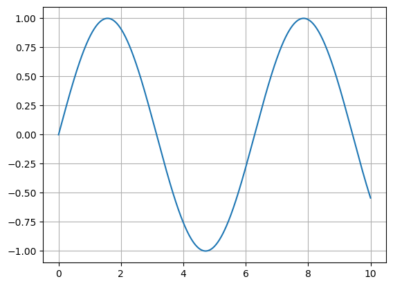
x = range(0, 10, length=1000);   or
x = LinRange(0, 10, 1000);  
1
0.0:0.01001001001001001:10.0
1
2
3
using PyPlot or Plots
grid()
plot(x, sin.(x))

png

1
2
1-element Array{PyCall.PyObject,1}:
 PyObject <matplotlib.lines.Line2D object at 0x140288630>

Discrete Convolution Using Circulant Matrix

$y[t] = h[t] * x[t]$ where $x[t] = [1, 2, 3, 0, -3, -1, 1, -2]$, $h[t] = [1, 3, 1]$

Use Julia LinearAlgebra for matrix/vector operation.
Use two space for new line.
Use DSP.conv to perform discrete convolution.
x: length=8; h: length=3; y: length=8+3-1=10 (padding two 0’s at x)

1
2
3
4
5
import Pkg; Pkg.add("SpecialMatrices")
using LinearAlgebra
using SpecialMatrices
using DSP
using FFTW
1
x = [1, 2, 3, 0,  -3, -1,  1, -2, 0, 0];
1
h = [1, 3, 1];
1
2
y = conv(x, h);
y'
1
2
1×12 Adjoint{Int64,Array{Int64,1}}:
 1  5  10  11  0  -10  -5  0  -5  -2  0  0

Circulant Matrix Multiplication Approximates Dicrete Convolution

First extend $h[t]$ by padding seven 0’s (10-3=7).
Use SpecialMatrices.Cirlulant to cyclic shift $h[t]$ and form a 10x10 Circulant matrix $\Phi$. Use SpecialMatrices.Matrix to convert special matrix type to normal Array

$y = \Phi x$

1
Φ = Matrix(Circulant([1,3,1,0,0,0,0,0,0,0]))
1
2
3
4
5
6
7
8
9
10
11
10×10 Array{Int64,2}:
 1  0  0  0  0  0  0  0  1  3
 3  1  0  0  0  0  0  0  0  1
 1  3  1  0  0  0  0  0  0  0
 0  1  3  1  0  0  0  0  0  0
 0  0  1  3  1  0  0  0  0  0
 0  0  0  1  3  1  0  0  0  0
 0  0  0  0  1  3  1  0  0  0
 0  0  0  0  0  1  3  1  0  0
 0  0  0  0  0  0  1  3  1  0
 0  0  0  0  0  0  0  1  3  1
1
2
y = Φ * x;
y'
1
2
1
2
1×10 Adjoint{Int64,Array{Int64,1}}:
 1  5  10  11  0  -10  -5  0  -5  -2

Find eigenvalues and eigenvectors of $\Phi$

$\Phi$ is a Circulant matrix, its eigenvalue array s[n] is “equivalent” to DFT($h[t]$), sort of,
up to frequency sequence difference.

For example, DFT frequency sequence is always defined counter clockwise on the unit circle (0,1,2,..,9) for n=10.
The eigenvalue/eigenvector decomposition: $\Phi = U P U^{*}$ In this eigvals implementation frequency is defined as conjugate first on the unit circle (0,1,9,2,8…,5)

The first eigenvalue of $\Phi$ corresponds to Nyquist frequency = 0 (DC: 1+1+3=5)
The last eigenvalue of $\Phi$ corresponds to Nyquist frequency = $\pi$ (highest AC: 1+1-3=-1)

Its eigenvector array P cosists of eigenvectors in column sequences.
The first column corresponds to DC eigenvector: [1, 1, …, 1]’.
The last column corresponds to DC eigenvector: [1, -1, …, -1]’.
image.png

1
s = eigvals(Φ)
1
2
3
4
5
6
7
8
9
10
11
10-element Array{Complex{Float64},1}:
                 5.0 + 0.0im               
  3.7360679774997863 + 2.7144122731725697im
  3.7360679774997863 - 2.7144122731725697im
   1.118033988749894 + 3.440954801177931im 
   1.118033988749894 - 3.440954801177931im 
 -0.7360679774997894 + 2.265384296592988im 
 -0.7360679774997894 - 2.265384296592988im 
 -1.1180339887498945 + 0.8122992405822655im
 -1.1180339887498945 - 0.8122992405822655im
 -1.0000000000000002 + 0.0im               
1
fft([1 3 1 0 0 0 0 0 0 0])'
1
2
3
4
5
6
7
8
9
10
11
10×1 Adjoint{Complex{Float64},Array{Complex{Float64},2}}:
                 5.0 - 0.0im               
    3.73606797749979 + 2.714412273172573im 
   1.118033988749895 + 3.4409548011779334im
 -0.7360679774997898 + 2.2653842965929876im
  -1.118033988749895 + 0.8122992405822659im
                -1.0 - 0.0im               
  -1.118033988749895 - 0.8122992405822659im
 -0.7360679774997898 - 2.2653842965929876im
   1.118033988749895 - 3.4409548011779334im
    3.73606797749979 - 2.714412273172573im 
1
P = Diagonal(s)
1
2
3
4
5
6
7
8
9
10
11
10×10 Diagonal{Complex{Float64},Array{Complex{Float64},1}}:
 5.0+0.0im          ⋅          …           ⋅                ⋅    
     ⋅      3.73607+2.71441im              ⋅                ⋅    
     ⋅              ⋅                      ⋅                ⋅    
     ⋅              ⋅                      ⋅                ⋅    
     ⋅              ⋅                      ⋅                ⋅    
     ⋅              ⋅          …           ⋅                ⋅    
     ⋅              ⋅                      ⋅                ⋅    
     ⋅              ⋅                      ⋅                ⋅    
     ⋅              ⋅             -1.11803-0.812299im       ⋅    
     ⋅              ⋅                      ⋅           -1.0+0.0im
1
2
U = eigvecs(Φ)
(round.(U*1000*sqrt(10)))/1000
1
2
3
4
5
6
7
8
9
10
11
10×10 Array{Complex{Float64},2}:
 1.0+0.0im   0.809+0.588im   0.809-0.588im  …  -0.809-0.588im   1.0+0.0im
 1.0+0.0im     1.0+0.0im       1.0-0.0im          1.0-0.0im    -1.0+0.0im
 1.0+0.0im   0.809-0.588im   0.809+0.588im     -0.809+0.588im   1.0+0.0im
 1.0+0.0im   0.309-0.951im   0.309+0.951im      0.309-0.951im  -1.0+0.0im
 1.0+0.0im  -0.309-0.951im  -0.309+0.951im      0.309+0.951im   1.0+0.0im
 1.0+0.0im  -0.809-0.588im  -0.809+0.588im  …  -0.809-0.588im  -1.0+0.0im
 1.0+0.0im    -1.0-0.0im      -1.0+0.0im          1.0-0.0im     1.0+0.0im
 1.0+0.0im  -0.809+0.588im  -0.809-0.588im     -0.809+0.588im  -1.0+0.0im
 1.0+0.0im  -0.309+0.951im  -0.309-0.951im      0.309-0.951im   1.0+0.0im
 1.0+0.0im   0.309+0.951im   0.309-0.951im      0.309+0.951im  -1.0+0.0im
1
2
U_b = inv(U)
(round.(U_b*1000*sqrt(10)))/1000
1
2
3
4
5
6
7
8
9
10
11
10×10 Array{Complex{Float64},2}:
    1.0+0.0im       1.0-0.0im    …     1.0+0.0im       1.0-0.0im  
  0.809-0.588im     1.0-0.0im       -0.309-0.951im   0.309-0.951im
  0.809+0.588im     1.0+0.0im       -0.309+0.951im   0.309+0.951im
 -0.809-0.588im   0.309-0.951im      0.309+0.951im  -0.809+0.588im
 -0.809+0.588im   0.309+0.951im      0.309-0.951im  -0.809-0.588im
 -0.809+0.588im  -0.309-0.951im  …   0.309-0.951im   0.809+0.588im
 -0.809-0.588im  -0.309+0.951im      0.309+0.951im   0.809-0.588im
 -0.809-0.588im     1.0+0.0im        0.309-0.951im   0.309+0.951im
 -0.809+0.588im     1.0-0.0im        0.309+0.951im   0.309-0.951im
    1.0-0.0im      -1.0+0.0im          1.0+0.0im      -1.0-0.0im  
1
(round.((U_b - U')*1000*sqrt(10)))/1000 # U_b is the same as conjugate transpose
1
2
3
4
5
6
7
8
9
10
11
10×10 Array{Complex{Float64},2}:
  0.0+0.0im   0.0-0.0im   0.0-0.0im  …  -0.0-0.0im  -0.0+0.0im   0.0-0.0im
  0.0+0.0im  -0.0-0.0im   0.0-0.0im      0.0+0.0im   0.0+0.0im   0.0+0.0im
  0.0-0.0im  -0.0+0.0im   0.0+0.0im     -0.0+0.0im   0.0-0.0im   0.0-0.0im
  0.0+0.0im  -0.0+0.0im  -0.0-0.0im      0.0-0.0im  -0.0+0.0im  -0.0+0.0im
  0.0-0.0im  -0.0-0.0im  -0.0+0.0im     -0.0+0.0im  -0.0-0.0im  -0.0-0.0im
  0.0-0.0im   0.0+0.0im   0.0+0.0im  …   0.0-0.0im  -0.0-0.0im   0.0+0.0im
  0.0+0.0im   0.0-0.0im   0.0-0.0im     -0.0+0.0im  -0.0+0.0im   0.0-0.0im
  0.0+0.0im  -0.0+0.0im   0.0-0.0im      0.0-0.0im   0.0-0.0im  -0.0+0.0im
  0.0+0.0im  -0.0-0.0im   0.0+0.0im      0.0+0.0im  -0.0+0.0im   0.0-0.0im
 -0.0-0.0im   0.0+0.0im  -0.0+0.0im     -0.0-0.0im   0.0+0.0im   0.0-0.0im
1
2
Phi = U * P * U_b  # verify U*P*U_b is the eigen value decompostion of Φ
real.(round.(Phi*1000))/1000
1
2
3
4
5
6
7
8
9
10
11
10×10 Array{Float64,2}:
  1.0  -0.0   0.0   0.0   0.0   0.0   0.0  -0.0   1.0   3.0
  3.0   1.0   0.0   0.0  -0.0  -0.0  -0.0   0.0  -0.0   1.0
  1.0   3.0   1.0   0.0   0.0   0.0   0.0   0.0  -0.0  -0.0
  0.0   1.0   3.0   1.0   0.0   0.0   0.0  -0.0  -0.0   0.0
  0.0   0.0   1.0   3.0   1.0   0.0   0.0  -0.0  -0.0   0.0
  0.0   0.0   0.0   1.0   3.0   1.0  -0.0   0.0   0.0   0.0
  0.0   0.0   0.0   0.0   1.0   3.0   1.0   0.0   0.0   0.0
  0.0   0.0   0.0  -0.0  -0.0   1.0   3.0   1.0  -0.0   0.0
 -0.0   0.0   0.0  -0.0   0.0   0.0   1.0   3.0   1.0  -0.0
  0.0   0.0  -0.0   0.0   0.0   0.0   0.0   1.0   3.0   1.0

Commutative Group - Translation Equivariant

  • Discrete convolution is equivalent to Circulant matrix multiplication.
  • Circulant matrix is itself commutative/Abelian group.
  • All Cirulant matrix multiplication can be decomposed into translation matrix multiplication’s superposition.
  • Discrete convolution is therefore translation multiplication commutable => translation equivariant
1
2
R = rand(10, 10)
Φ * R - R * Φ   # Random matrix multiplication does NOT commutate with Circulant matrix
1
2
3
4
5
6
7
8
9
10
11
10×10 Array{Float64,2}:
 -1.58559   -0.237127  -0.129967  …   0.066688  -1.72504    -1.40459 
  1.04033    1.08089    0.34026      -0.782441  -1.91891    -1.63573 
  3.35632    0.831891   0.805718     -0.849477   1.18107     0.183805
  0.815998  -1.54383   -0.38105      -1.00838   -0.141359   -0.176457
 -0.915783   0.225814  -1.14518       0.5001     0.128517    1.68327 
 -2.07181    1.04074   -2.12622   …   1.62098    0.348925    1.07887 
  0.313094   1.84738   -0.894152      0.282517  -2.32041    -0.039078
  1.11406   -0.71119   -1.059        -0.981632  -0.0110641   0.999691
  1.42449   -1.50675   -1.53478       1.06594    0.590891    2.41234 
 -2.2159    -2.33044   -1.29612       0.626618  -0.119957    0.743334
1
Tg = Circulant([1,2,3,4,5,6,7,8,9,10]) # Verify Circulant matrix multiplication is a commutative group
1
2
3
4
5
6
7
8
9
10
11
10×10 Circulant{Int64}:
  1  10   9   8   7   6   5   4   3   2
  2   1  10   9   8   7   6   5   4   3
  3   2   1  10   9   8   7   6   5   4
  4   3   2   1  10   9   8   7   6   5
  5   4   3   2   1  10   9   8   7   6
  6   5   4   3   2   1  10   9   8   7
  7   6   5   4   3   2   1  10   9   8
  8   7   6   5   4   3   2   1  10   9
  9   8   7   6   5   4   3   2   1  10
 10   9   8   7   6   5   4   3   2   1
1
Φ * Tg - Tg * Φ   
1
2
3
4
5
6
7
8
9
10
11
10×10 Array{Int64,2}:
 0  0  0  0  0  0  0  0  0  0
 0  0  0  0  0  0  0  0  0  0
 0  0  0  0  0  0  0  0  0  0
 0  0  0  0  0  0  0  0  0  0
 0  0  0  0  0  0  0  0  0  0
 0  0  0  0  0  0  0  0  0  0
 0  0  0  0  0  0  0  0  0  0
 0  0  0  0  0  0  0  0  0  0
 0  0  0  0  0  0  0  0  0  0
 0  0  0  0  0  0  0  0  0  0
1
g = Circulant([0,1,0,0,0,0,0,0,0,0])  # Circulant matrix group generator: right cyclic shift by 1
1
2
3
4
5
6
7
8
9
10
11
10×10 Circulant{Int64}:
 0  0  0  0  0  0  0  0  0  1
 1  0  0  0  0  0  0  0  0  0
 0  1  0  0  0  0  0  0  0  0
 0  0  1  0  0  0  0  0  0  0
 0  0  0  1  0  0  0  0  0  0
 0  0  0  0  1  0  0  0  0  0
 0  0  0  0  0  1  0  0  0  0
 0  0  0  0  0  0  1  0  0  0
 0  0  0  0  0  0  0  1  0  0
 0  0  0  0  0  0  0  0  1  0
1
g*g  # right cyclic shift by 2
1
2
3
4
5
6
7
8
9
10
11
10×10 Array{Int64,2}:
 0  0  0  0  0  0  0  0  1  0
 0  0  0  0  0  0  0  0  0  1
 1  0  0  0  0  0  0  0  0  0
 0  1  0  0  0  0  0  0  0  0
 0  0  1  0  0  0  0  0  0  0
 0  0  0  1  0  0  0  0  0  0
 0  0  0  0  1  0  0  0  0  0
 0  0  0  0  0  1  0  0  0  0
 0  0  0  0  0  0  1  0  0  0
 0  0  0  0  0  0  0  1  0  0
1
2
eye = 1.0*Matrix(I, 10, 10)   # Verify Circulant Tg is decomposed into group generator superposition
1*eye+2*g+3*g*g+4*g*g*g+5*g*g*g*g+6*g*g*g*g*g+7*g*g*g*g*g*g+8*g*g*g*g*g*g*g+9*g*g*g*g*g*g*g*g+10*g*g*g*g*g*g*g*g*g
1
2
3
4
5
6
7
8
9
10
11
10×10 Array{Float64,2}:
  1.0  10.0   9.0   8.0   7.0   6.0   5.0   4.0   3.0   2.0
  2.0   1.0  10.0   9.0   8.0   7.0   6.0   5.0   4.0   3.0
  3.0   2.0   1.0  10.0   9.0   8.0   7.0   6.0   5.0   4.0
  4.0   3.0   2.0   1.0  10.0   9.0   8.0   7.0   6.0   5.0
  5.0   4.0   3.0   2.0   1.0  10.0   9.0   8.0   7.0   6.0
  6.0   5.0   4.0   3.0   2.0   1.0  10.0   9.0   8.0   7.0
  7.0   6.0   5.0   4.0   3.0   2.0   1.0  10.0   9.0   8.0
  8.0   7.0   6.0   5.0   4.0   3.0   2.0   1.0  10.0   9.0
  9.0   8.0   7.0   6.0   5.0   4.0   3.0   2.0   1.0  10.0
 10.0   9.0   8.0   7.0   6.0   5.0   4.0   3.0   2.0   1.0
1
(Φ*(Tg*x) - Tg*(Φ*x) )'    # Φ and Tg are commutative on input signal x as expected
1
2
1
2
1×10 Adjoint{Int64,Array{Int64,1}}:
 0  0  0  0  0  0  0  0  0  0
1
(Φ*x)'   # normal discrete convolution
1
2
1
2
1×10 Adjoint{Int64,Array{Int64,1}}:
 1  5  10  11  0  -10  -5  0  -5  -2
1
(g*(Φ*x))'   # group generator causes discrete convolution right cyclic translation
1
2
1
2
1×10 Adjoint{Int64,Array{Int64,1}}:
 -2  1  5  10  11  0  -10  -5  0  -5
1
(g*x)'    # group generator's action on x[t] is to right cyclic shift by 1
1
2
1×10 Adjoint{Int64,Array{Int64,1}}:
 0  1  2  3  0  -3  -1  1  -2  0
1
(Φ*(g*x))'  # discrete convolution of the right cyclic shift signal
1
2
1
2
1×10 Adjoint{Int64,Array{Int64,1}}:
 -2  1  5  10  11  0  -10  -5  0  -5
1
(Φ*(g*x) - g*(Φ*x) )'   # discrete convolution is translation (i.e. g or g*g or g*g*g ...) eqivaraint (commutative)
1
2
1
2
1×10 Adjoint{Int64,Array{Int64,1}}:
 0  0  0  0  0  0  0  0  0  0
1