Edge AI Trilogy III - Model Compression

Edge AI 三部曲的最終篇是 model compression. 之後還會有番外篇 on advance topics such as NAS, etc. 為什麼 model compression 放在最終篇？可以用 Han Song 的 deep compression [@hanDeepCompression2016; @hanLearningBoth2015] 為例。下圖架構正好對應三部曲：pruning, quantization, and (parameter) compression.

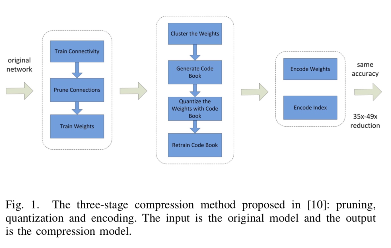
基本上 parameter compression 可以收割之前 sparsity, quantization, weight sharing 帶來的 storage and memory bandwidth reduction (35x-49x) 的好處。當然隨著 parameter reduction, 額外還有 computation and energy reduction 的好處，例如 zero-skipping for sparsity 和 low bitwidth MAC computation for quantization and weight sharing.

Model compression 包含 parameter compression 以及其他的技巧減少 parameter, 甚至改變 model structure。最後的 model size (in MB) and MAC (in GFlop) 就是 “moment of the truth”. 就像 SNR or BER 是通訊系統的整體檢驗。除了 parameter pruning (sparsity) and sharing (clustering and quantizing) 之外，[@chengSurveyModel2019] 把 model compression 作法分為四類：

Theme Name	Description	Applications	Details
Parameter pruning and sharing	Reducing redundant parameters not sensitive to the performance	CONV and FC layer	Robust to various settings, can achieve good performance, support both train from scratch and pre-trained model
Low-rank factorization	Using matrix/tensor decomposition to estimate the informative parameters	CONV and FC layer	Standardized pipeline, easily to implement, support both train from scratch and pre-trained model
Transferred/compact convolutional filters	Designing special structural convolutional filters to save parameters	CONV layer only	Algorithms are dependent on applications, usually achieve good performance, only support train from scratch
Knowledge distillation	Training a compact neural network with distilled knowledge of a large model	CONV and FC layer	Model performances are sensitive to applications and network structure only support train from scratch

Another paper 提出的 model compression 分類 [@kuzminTaxonomyEvaluation2019].

• SVD-based methods (low rank)
• Tensor decomposition-based methods (low rank)
• Pruning methods
• Compression ratio selection method
• Loss-aware compression
• Probabilistic compression
• Efficient architecture design

Another good review paper from Purdue. [@goelSurveyMethods2020]

Technique	Description	Advantages	Disadvantages
Quantization and Pruning	Reduces precision/completely removes the redundant parameters and connections from a DNN.	Negligible accuracy loss with small model size. Highly efficient arithmetic operations.	Difficult to implement on CPUs and GPUs because of matrix sparsity. High training costs.
Filter Compression and Matrix Factorization	Decreases the size of DNN filters and layers to improve efficiency.	High accuracy. Compatible with other optimization techniques.	Compact convolutions can be memory inefficient. Matrix factorization is computationally expensive.
Network Architecture Search	Automatically finds a DNN architecture that meets performance and accuracy requirements on a target device.	State-of-the-art accuracy with low energy consumption.	Prohibitively high training costs.
Knowledge Distillation	Trains a small DNN with the knowledge of a larger DNN to reduce model size.	Low computation cost with few DNN parameters.	Strict assumptions on DNN structure. Only compatible with softmax outputs.

Model => Data => Memory?? (from Huawei’s talk)

My classification:

Level 1: Compression Without changing the network layer and architecture, i.e. weight compression including pruning (weight = 0), quantization (reduce weight bitwidth), weight sharing, etc. 可以到達 10x-50x compression for large network (e.g. resnet, alexnet, etc.)

Level 2: Modify network architecture based on some basic rules (matrix/tensor decomposition), network fusion, etc.

Level 3: Change the network architecture completely. Knowledge transfer (KT) or knowledge distillation (KD) belongs to Level 3 or Level 4?

Level 4: Network architecture search (NAS) to explore a big search space and based on the constraints of edge device capability. 嚴格來說，已經不是 model compression, 而是 model search or exploration.

Level 1: Quantization and Pruning and Huffman Encode

Details 可以參考之前兩篇文章。

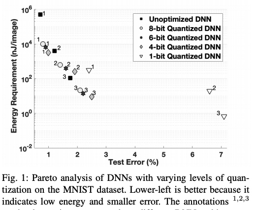
In summary, quantization from FP32 to INT8 可以 save up to 75% (4x) storage/bandwidth/computation, 而不損失 accuracy or increase error. 這也代表更低的功耗。如果使用更少 bitwidth (6/4/2/1), 可以省更多，但是可能 trade-off accuracy/error 或是限制應用的範圍。下圖是不同 quantized bitwidth 對應的 energy vs. test error.

Pruning 是另一個更深奧更有空間的方式。可以視為 quantization 的 special case (weight and activation = 0), 但更進一步是一個 subset network 可以完全 represent the original network (lottery conjecture). pruning 對於一些 “fat network” 可以達到 10x 的 saving. 對於一些 “lean network”, e.g. MobileNet 就比較少 saving.

Parameter compression 也是常用的技巧。包含 weight compression and activation compression.
Parameter compression 省最多是 data 包含很多的冗余或是 regular structure，例如大量的 0, 從 information theory 就是 low entropy facilitate compression. Huffman encoding 是一個有效的方法 for parameter compression.

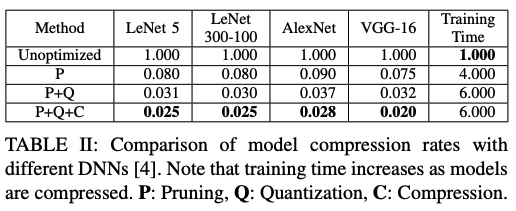pruning, quantization, compression 可以合在一起得到最佳的效果 at a cost of higher training time.

Level 2: Matrix and Tensor Decomposition

分為兩個部分: CONV layer 和 FC layer. 當然廣義來說，FC layer 也是一種 CONV layer with kernel size WxHxC. 此處 CONV layer 的 kernel size 一般指 1x1, 3x3, …, 11x11, etc.

對於 CONV layer, 越大 kernel filter 的 parameters and MACs 越大，較小的 kernel filter 的 parameters and MACs 越小。但如果把所有大的 kernel filter 都替換成小的 kernel filter, 會影響 DNN 的平移不變性，這會降低 DNN model 的精度。因此一些策略是識別冗余的 kernel filter, 並用較小 kernel filter 取代。例如 VGG 把所有大於 3x3 (e.g. 5x5, 7x7, etc.) 都用 3x3 filter 取代。SqueezeNet and MobileNet 甚至用 1x1 取代部分的 3x3 filter.

Convolutional Filter Compression (CONV layer only)

SqueezeNet use 1x1 kernel to replace 3x3 kernel filter. MobileNet use depth-wise + point-wise (1x1) network to replace original kernel to reduce computation by 1/8-1/9 for 3x3 kernel.

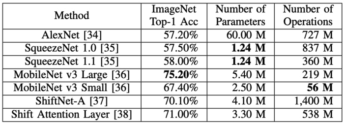MobileNet v3 可以達到不錯的精度 (75%)，但是 parameter and MAC 比起 AlexNet 少非常多。比起 ResNet50 (parameter 25M, MAC 4G) 也好不少。

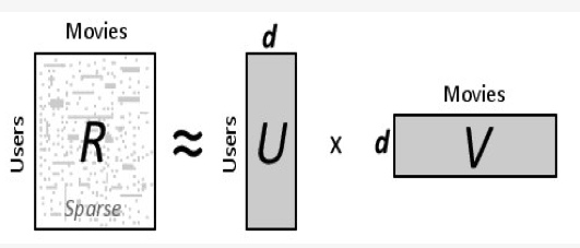
Matrix Factorization/Decomposition (CONV or FC layer)

通過將張量或矩陣分解為合積形式（sum-product form），將多維張量分解為更小的矩陣，從而可以消除冗余計算。一些因子分解方法可以將DNN模型加速4 倍以上，因為它們能夠將矩陣分解為更密集的參數矩陣，且能夠避免非結構化稀疏乘法的局部性問題。

目前 Matrix decomposition/factorization 並非主流。原因：

• 關於矩陣分解，有多種技術。Kolda等人證明，大多數因子分解技術都可以用來做DNN模型的加速，但這些技術在精度和計算複雜度之間不一定能夠取得最佳的平衡。
• 由於缺乏理論解釋，因此很難解釋為什麼一些分解（例如CPD、BMD）能夠獲得較高的精度，而其他分解卻不能。
• 與矩陣分解相關的計算常常與模型獲得的性能增益相當，造成收益與損耗抵消。
• 矩陣分解很難在大型DNN模型中實現，因為隨著深度增加分解超參會呈指數增長，訓練時間主要耗費在尋找正確的分解超參。

更多更 detailed description 可以參考 [@kuzminTaxonomyEvaluation2019].

Level 3: Knowledge Transfer or Distillation

https://www.leiphone.com/news/202003/cggvDDPFIVTjydxS.html 大模型比小模型更準確，因為參數越多，允許學習的函數就可以越複雜。那麼能否用小的模型也學習到這樣複雜的函數呢？

一種方式便是知識遷移（KT, Knowledge Transfer），通過將大的DNN模型獲得的知識遷移到小的DNN模型上。為了學習複雜函數，小的 DNN 模型會在大的 DNN 模型標記處的數據上進行訓練。其背後的思想是，大的 DNN 標記的數據會包含大量對小的DNN有用的信息。例如大的 DNN 模型對一個輸入圖像在一些類標籤上輸出中高機率，那麼這可能意味著這些類共享一些共同的視覺特徵；對於小的 DNN模型，如果去模擬這些機率，相比於直接從數據中學習，要能夠學到更多。

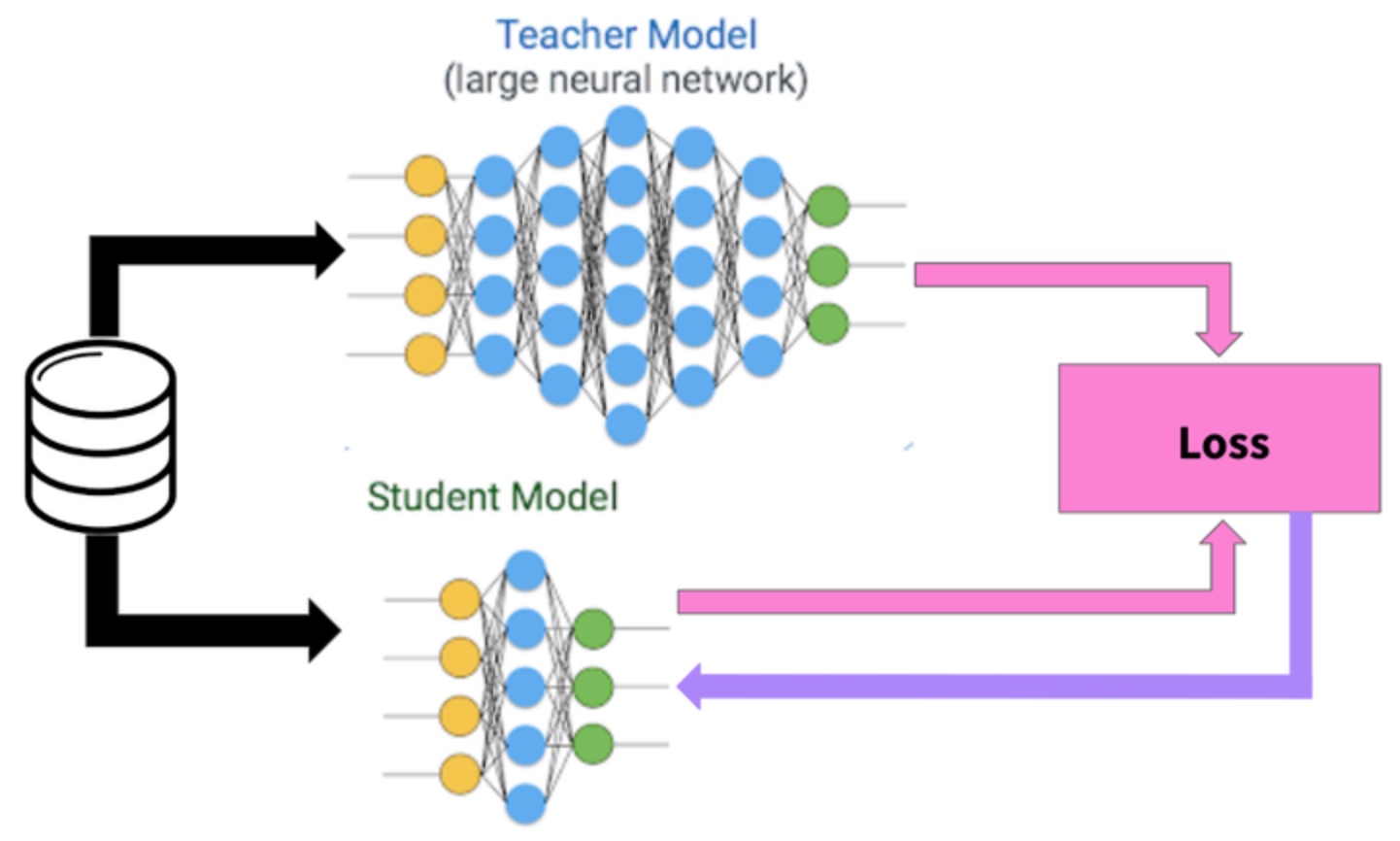
具體的作法之一是 Hinton 在 2014年 提出的知識蒸餾 (KD, Knowledge Distillation)，這種方法的訓練過程相比於知識遷移 (KT) 要簡單得多。在知識蒸餾中，小的 DNN 模型使用學生-教師模式進行訓練，其中小的 DNN 模型是學生，一組專門的 DNN 模型是教師；通過訓練學生，讓它模仿教師的 softmax 輸出，小的DNN 模型可以完成整體的任務。但在 Hinton 的工作中，小的 DNN 模型的準確度卻相應有些下降。 Li 等人利用最小化教師與學生之間特徵向量的歐氏距離，進一步提高的小的 DNN 模型的精度。類似的，FitNet 讓學生模型中的每一層都來模仿教師的特徵圖。但以上兩種方法都要求對學生模型的結構做出嚴格的假設，其泛化性較差。

Knowledge transfer/distillation is very interesting and similar to proxy AI I thought before!

Knowledge transfer or distillation 是個非常有趣而且實用的技術。例如 teacher model 可以是雲端的大 DNN 模型，有比較好的精度以及泛化性。但在 edge or device 可以 deploy student model, i.e. 小 DNN 模型。雖然精度和泛化性比較差，但是 quick response, 以及 edge and device 不一定需要非常強的泛化性 (e.g. local voice recognition, or local face detection).

優點：基於知識遷移和知識蒸餾的技術可以顯著降低大型預訓練模型的計算成本。有研究表明，知識蒸餾的方法不僅可以在計算機視覺中應用，還能用到許多例如半監督學習、域自適應等任務中。

缺點及改進方向：知識蒸餾通常對學生和教師的結構和規模有嚴格的假設，因此很難推廣到所有的應用中。此外目前的知識蒸餾技術嚴重依賴於 softmax 輸出，不能與不同的輸出層協同工作。作為改進方向，學生可以學習教師模型的神經元激活序列，而不是僅僅模仿教師的神經元/層輸出，這能夠消除對學生和教師結構的限制（提高泛化能力），並減少對softmax輸出層的依賴。

Transfer learning is different from knowledge transfer/distillation

The objective of transfer learning and knowledge distillation are quite different. In transfer learning, the weights are transferred from a pre-trained network to a new network and the pre-trained network should exactly match the new network architecture. What this means is that the new network is essentially as deep and complex as the pre-trained network.

the objective of knowledge distillation is different. The aim is not to transfer weights but to transfer the generalizations of a complex model to a much lighter model. 如何 transfer generalizations? 使用 student-teach model 是一種方式。還有其他的方式可以參考 [@kompellaTapDark2018].

Level 4: Network Architecture Search (NAS)

在設計低功耗計算機視覺程序時，針對不同的任務可能需要不同的DNN模型架構。但由於存在許多這種結構上的可能性，通過手工去設計一個最佳DNN模型往往是困難的。最好的辦法就是將這個過程自動化，即網絡架構搜索技術（Network Architecture Search）。

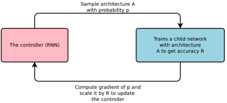
NAS使用一個遞歸神經網絡(RNN)作為控制器，並使用增強學習來構建候選的DNN架構。對這些候選DNN架構進行訓練，然後使用驗證集進行測試，測試結果作為獎勵函數，用於優化控制器的下一個候選架構。

NASNet 和AmoebaNet 證明瞭NAS的有效性，它們通過架構搜索獲得DNN模型能夠獲得SOTA性能。

為了獲得針對移動設備有效的DNN模型，Tan等人提出了MNasNet，這個模型在控制器中使用了一個多目標獎勵函數。在實驗中，MNasNet 要比NASNet快2.3倍，參數減少4.8倍，操作減少10倍。此外，MNasNet也比NASNet更準確。

不過，儘管NAS方法的效果顯著，但大多數NAS算法的計算量都非常大。例如，MNasNet需要50,000個GPU 時才能在ImageNet數據集上找到一個高效的DNN架構。

為了減少與NAS相關的計算成本，一些研究人員建議基於代理任務和獎勵來搜索候選架構。例如在上面的例子中，我們不選用ImageNet，而用更小的數據集CIFAR-10。FBNet正是這樣來處理的，其速度是MNasNet的420倍。但Cai等人表明，在代理任務上優化的DNN架構並不能保證在目標任務上是最優的，為了克服基於代理的NAS解決方案所帶來的局限性，他們提出了Proxyless-NAS，這種方法會使用路徑級剪枝來減少候選架構的數量，並使用基於梯度的方法來處理延遲等目標。他們在300個GPU時內便找到了一個有效的架構。此外，一種稱為單路徑NAS（Single-Path NAS）的方法可以將架構搜索時間壓縮到 4 個GPU時內，不過這種加速是以降低精度為代價的。

優點：NAS通過在所有可能的架構空間中進行搜索，而不需要任何人工干預，自動平衡準確性、內存和延遲之間的權衡。NAS能夠在許多移動設備上實現準確性、能耗的最佳性能。

缺點及改進方向：計算量太大，導致很難去搜索大型數據集上任務的架構。另外，要想找到滿足性能需求的架構，必須對每個候選架構進行訓練，並在目標設備上運行來生成獎勵函數，這會導致較高的計算成本。其實，可以將候選DNN在數據的不同子集上進行並行訓練，從而減少訓練時間；從不同數據子集得到的梯度可以合併成一個經過訓練的DNN。不過這種並行訓練方法可能會導致較低的準確性。另一方面，在保持高收斂率的同時，利用自適應學習率可以提高準確性。

Model Compression Examples

Ex1: Deep Compression by Han (Level 1)

參考 fig.1 使用 pruning, quantization, and parameter compression. 整體的效益如下。精度和 AlexNet 差不多 (TBC)。

• Step 1: Pruning (9x-13x)
• Step 2: Quantizing clustered weights for weight sharing (32bit -> 5bit) (~4x)
• Step 3: Compression: encode weights/index for weight compression; Huffman encoding sparsity/zero and weight sharing compression.
• Total: 35x-49x

Accuracy result (TBA)

Ex2: Model compression via distillation and quantization (Level 1+3)

This excellent paper [@polinoModelCompression2018] ¹ proposes two new compression methods, which jointly leverage weight quantization and distillation of larger networks, called “teachers,” into compressed “student” networks. 簡單說 FP32 model 是 teacher model; quantized model 是 student model. Github code ².

The first method is called quantized distillation and leverages distillation during the training process, by incorporating distillation loss, expressed with respect to the teacher network, into the training of a smaller student network whose weights are quantized to a limited set of levels. teacher model 使用 FP32 deep model; student model 則是 uniformly quantized and shallow model. 藉著 distillation loss that teacher model can train student model.

The second method, differentiable quantization, optimizes the location of quantization points through stochastic gradient descent, to better fit the behavior of the teacher model. 使用和 student model 同樣的小模型。重點是 linear but non-uniform quantization. 但沒有 distillation loss; 而是用一般的 cross-entropy loss to train this model and optimize the non-uniform quantization. 當然也可以使用 non-uniform quantization for student model. 可能 computation 會太複雜。

其他細節請參考[@polinoModelCompression2018]. 這裏直接討論結果。

CIFAR10 accuracy. Teacher model: 5.3M param of FP32, 21MB, accuracy 89.71%.

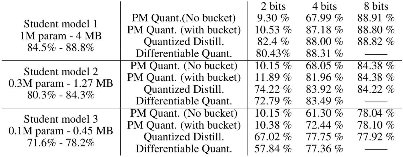
• 有三種 student models, 分別為 1M/0.3M/0.1M param 如下表左第一欄。

• 第一欄 (A) 都是 FP32 full precision training. 例如 A1 代表 student model 1, 1M param, FP32：4MB. 兩個 accuracy 對應 cross-entropy loss and distillation loss. Accuracy 84.5% 對應 normal training (cross-entropy loss). Accuracy 88.8% 對應 teacher-student training (distillation loss).

• 第二欄 (B) 都是 quantized training. PM (post-mortem) Quant. 只是把 FP32 teacher-student training 的 weight 直接 post training uniform quantization without any additional operation. 有兩種 PM Quant., 一是 global scaling (no bucket), 另一個是 local scaling (with bucket size = 256). 所以 (1) PM Quant. accuracy 一定差於 FP32 accuracy (88.8%). Quantized Distill. 使用 distillation loss back propagation, 因此 accuracy is better than PM Quant. In summary, FP Distill. > Quantized Distill. > PM (with bucket) > PM (no bucket)

• Differentiable Quant. 使用 cross-entropy loss training. 從另一個角度, non-uniform quantization, approach this problem. 在 4-bits quantization 的表現不輸於 uniform distillation loss training. 但在 2-bits quantization distillation loss training 還是比較好。合理推論，differentiable non-uniform quantization with distillation loss 應該會有最佳的 accuracy.

• Differentiable quantization 在 computation 不容易在 edge AI 實現，因為 quantized values 不會落在 linear grid 上，很難用 finite bitwidth 表示，也很難做 MAC 計算。比較接近的解法是用 k-mean clustering algorithm to cluster weights and adopt the centroids as quantization points. Han 稱為 weight sharing.
• 最佳的結果 assuming accuracy loss < 2% compared with baseline (89.71%) is student model 1 (1M param) of 4-bit with accuracy 88%. The total size of best student model 1 is: 1M param x 0.5 = 0.5MB. A factor of 21MB/0.5MB = 42x saving in memory/bandwidth/computation etc.!!!

更好的結果是用比較 deeper student model, 但是用 4-bit (5.8M x 0.5 = 2.9MB), 而且 accuracy 還比較好 (92.3% vs. 89.71%). A factor of 21MB/2.9MB = 7.2x saving in memory/bandwidth/computation etc.!!!

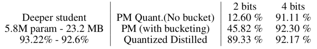
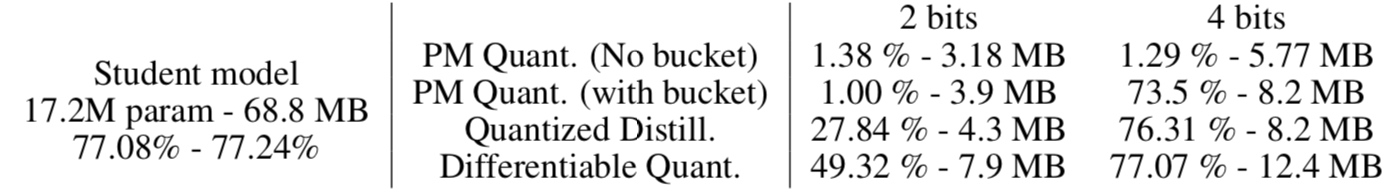
CIFAR100 accuracy. Teacher model: 36.5M param of FP32, 146MB, accuracy 77.21%.

• Student model is 17.2M param, about 1/2 of teacher model. 4-bit model is 8.2MB with accuracy 76.31%. A factor of 146MB/8.2MB = 17.8x saving.
• Differential quantization seems to perform better, but with more params and more complicated computation.

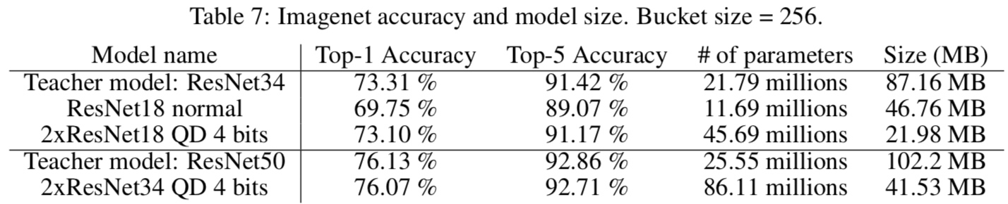
Imagenet accuracy. Teacher model: ResNet34 or ResNet50

• Student model: 2xResNet18 QD 4 bit and 2xResNet34 QD 4 bit
• Student model of 4-bit 可以得到和 teacher model 類似 accuracy. 但 size 比起 teacher FP32 model 少了 2x-4x.

Distillation + Quantization 結論：

• FP32 to INT8 已經有很多 post-training quantization or quantization aware training 可以達到同樣的 accuracy. 因此 4x saving 已經很普通。
• Teacher-student models 在小 dataset (CIFAR10), model compression 效果比較突出: (1) 8x from FP32 to 4-bit; (2) student model 可以比 teacher model gain 4x-5x. 但對於大 dataset, CIFAR100 or ImageNet, student model param 已經接近甚至超過 teacher model param. 此時只有 FP32 to 4-bit gain.
• 對於大 dataset, knowledge distillation 的結果並不突出。

Summary

• Level 1 + Level 2 compression 可以同時使用。增加壓縮的倍率。
• Level 1 + Level 3 compression 可以同時使用。對於大 dataset 效果有限。但是小 dataset 似乎不錯。
• Level 4 NAS 雖然看起來很好，但是需要太多的 computation resource/time to search. 需要更好的方式用於 edge AI.

Reference

Cheng, Yu, Duo Wang, Pan Zhou, and Tao Zhang. 2019. “A Survey of Model Compression and Acceleration for Deep Neural Networks,” September. https://arxiv.org/abs/1710.09282v8.

Goel, Abhinav, Caleb Tung, Yung-Hsiang Lu, and George K. Thiruvathukal. 2020. “A Survey of Methods for Low-Power Deep Learning and Computer Vision,” March. http://arxiv.org/abs/2003.11066.

Han, Song, Huizi Mao, and William J. Dally. 2016. “Deep Compression: Compressing Deep Neural Networks with Pruning, Trained Quantization and Huffman Coding,” February. http://arxiv.org/abs/1510.00149.

Han, Song, Jeff Pool, John Tran, and William J. Dally. 2015. “Learning Both Weights and Connections for Efficient Neural Networks,” October. http://arxiv.org/abs/1506.02626.

Kompella, Ravindra. n.d. “Tap into the Dark Knowledge Using Neural Nets Distillation.” Medium. Accessed April 2, 2020. https://towardsdatascience.com/knowledge-distillation-and-the-concept-of-dark-knowledge-8b7aed8014ac.

Kuzmin, Andrey, Markus Nagel, Saurabh Pitre, Sandeep Pendyam, Tijmen Blankevoort, and Max Welling. 2019. “Taxonomy and Evaluation of Structured Compression of Convolutional Neural Networks,” December. http://arxiv.org/abs/1912.09802.

Polino, Antonio, Razvan Pascanu, and Dan Alistarh. 2018. “Model Compression via Distillation and Quantization,” February. http://arxiv.org/abs/1802.05668.

1. Published in ICLR 2018 ↩

2. https://github.com/antspy/quantized_distillation ↩