Main Reference
- [@poczosCllusteringEM2015]
- [@matasExpectationMaximization2018] good reference
- [@choyExpectationMaximization2017]
- [@tzikasVariationalApproximation2008] excellent introductory paper
Maximum Likelihood Estimation (MLE) 和應用
Maximum likelihood estimation (MLE) 最大概似估計是一種估計模型參數的方法。適用時機在於手邊有模型,但是模型參數有無限多種,透過真實觀察到的樣本資訊,想辦法導出最有可能產生這些樣本結果的模型參數,也就是挑選使其概似性(Likelihood)最高的一組模型參數,這系列找參數的過程稱為最大概似估計法。
Bernoulli distribution:投擲硬幣正面的機率 $\theta$, 反面的機率 $1-\theta$. 連續投擲的正面/反面的次數分別是 H/T. Likelihood function 為
\[f(\theta, H, T)=\theta^{H}(1-\theta)^{T}\]MLE 在無限個 $\theta$ 中,找到一個使概似性最大的 $\theta$, i.e. $\widehat{\theta}_{\mathrm{MLE}} =\arg \max _{\theta} {\theta^{H}(1-\theta)^{T}}$
只要 likelihood function 一次微分,可以得到
\[\widehat{\theta}_{M L E}=\frac{H}{T+H}\]就是平均值,推導出來的模型參數符合直覺。
Normal distribution: 假設 mean unknown, variance known, 我們可以用 maximum log-likelihood function
\[\underset{\mu}{\operatorname{argmax}} f\left(x_{1}, \ldots, x_{n}\right) \Rightarrow \underset{\mu}{\operatorname{argmax}} \log f\left(x_{1}, \ldots, x_{n}\right)\] \[\begin{aligned} &\frac{\mathrm{d}}{d \mu}\left(\sum_{i=1}^{n}-\frac{\left(x_{i}-\mu\right)^{2}}{2 \sigma^{2}}\right)=\sum_{\mathrm{i}=1}^{\mathrm{n}} \frac{\left(x_{i}-\hat{\mu}\right)}{\sigma^{2}}=\sum_{i=1}^{n} x_{i}-n \hat{\mathrm{u}}=0 \\ &\hat{\mu}=\overline{\mathrm{X}}=\frac{\sum_{i=1}^{n} x_{i}}{n} \end{aligned}\]微分的結果告訴我們,樣本的平均值,其實就是母體平均值 $\mu$ 最好的估計!又是一個相當符合直覺的答案,似乎 MLE 只是用來驗證直覺的工具。
這是一個錯覺,常見的 distribution (e.g. Bernoulli, normal distribution) 都是 exponential families. 可以證明 maximum log-likelihood functions of exponential families 都是 concave function, 沒有 local minimum. 非常容易用數值方法找到最佳解,而且大多有 analytical solution.
但只要 distribution function 更複雜一點,例如兩個 normal/Gaussian distribution weighted sum to 1, MLE 就非常難解。稱為 Gaussian mixture model (GMM) with 2 groups, GMM(2).
另一種情況:MLE 雖然直接明瞭,但現實常常會遇到 missing data 或是 hidden data/state (state 也視為 data). 此時就需要 Expectation Maximization (EM) algorithm.
例如 GMM(2) 可以視為有一個 hidden state $z$ with binary value, $p(x) = p(x\mid z=0) p(z=0) + p(x\mid z=1) p(z=1)$. $p(x\mid z=0)$ 和 $p(x\mid z=1)$ 分別是不同 normal distributions.
以下先 Q&A maximum likelihood estimation (MLE) vs. expectation maximization (EM) 兩種算法。其實是視 EM 為 MLE 的推廣。 接著用四個簡單例子 (toy example) 說明 MLE 如何推廣到 EM.
Q&A of MLE Versus EM
Q: Why EM is a special case of MLE?
- If the problem can be formulated as MLE parameter estimation of incomplete/hidden data. Then EM algorithm 的 E-step is guessing incomplete/hidden data; M-step 就對應 MLE parameter estimation with modification (見本文後段)。
- EM M-Step is essentially a MLE parameter estimation with modification.
- EM can be seen as an iterative MLE. EM may converge at local minimum during iteration.
Q: How EM can be used for to parameter estimation and incomplete/hidden data estimation?
- For Bayesian, 兩者可以視為同一類。Unknown parameters 亦可以視為 missing data with distribution. 此時 EM algorithm 相當于 2D coordinate descent (energy) optimization [@wikiCoordinateDescent2021], different from gradient descent. EM 的 E-step 對應 (conditional) distribution coordinate descent; M-step 對應 parameter coordinate descent.
- For Frequentist (古典統計), E-step is guessing incomplete/hidden data; M-step 就對應 MLE parameter estimation.
Toy Example [@matasExpectationMaximization2018]
前提摘要
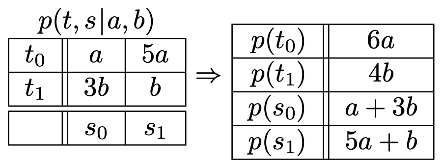
一個簡單例子觀察 temperature and amount of snow (溫度和雪量, both are binary input) 的 joint probability depending on two “scalar factors” $a$ and $b$ as $p(t, s | a, b)$
| $s_0$ | $s_1$ | |
|---|---|---|
| $t_0$ | $a$ | $5a$ |
| $t_1$ | $3b$ | $b$ |
注意 $a$ and $b$ are parameters, 不是 conditional probability. 另外因為機率和為 1 做為一個 constraint: $6a + 4b = 1$
例一: MLE
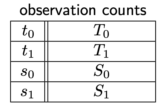
一個 ski-center 觀察 $N$ 天的溫度和雪量得到以下的統計,$N_{ij} \in \mathbf{I}$, 如何估計 $a$ and $b$?
| $s_0$ | $s_1$ | |
|---|---|---|
| $t_0$ | $N_{00}$ | $N_{01}$ |
| $t_1$ | $N_{10}$ | $N_{11}$ |
Likelihood function (就是 joint pdf of $N$ repeat experiments)
\[P(\mathcal{T} \mid a, b)= C a^{N_{00}}(5 a)^{N_{01}}(3 b)^{N_{10}}(b)^{N_{11}}\]where $C = (\Sigma N_{ij})! / \Pi (N_{ij}!)$ 是 MLE 無關的常數
問題改成 maximum log-likelihood with constraint and $C’ = \ln C$
\[L(a, b, \lambda) = C' + N_{00} \ln a+N_{01} \ln 5 a+N_{10} \ln 3 b+N_{11} \ln b+\lambda(6 a+4 b-1)\] \[\begin{gathered} \frac{\partial L}{\partial a}=N_{00} \frac{1}{a}+N_{01} \frac{1}{a}+6 \lambda=0 \\ \frac{\partial L}{\partial b}=N_{10} \frac{1}{b}+N_{11} \frac{1}{b}+4 \lambda=0 \\ \frac{\partial L}{\partial \lambda}=6 a+4 b - 1 = 0 \end{gathered}\]上述方程式的解為 \(a=\frac{N_{00}+N_{01}}{6 N} \quad b=\frac{N_{10}+N_{11}}{4 N} \quad \lambda = -(N_{00}+N_{01}+N_{10}+N_{11})=-N\)
結果很直觀。其實就是利用大數法則: $a\cdot N \sim N_{00}; 5a\cdot N\sim N_{01}; 3b\cdot N\sim N_{10}; b\cdot N\sim N_{11}$ 再來大數法則 (a+5a)N~N00+N01; (3b+b)N~N10+N11 => a = .. ; b = …
例二 incomplete/hidden Data
假設我們無法觀察到完整的”溫度和雪量“;而是“溫度或雪量”,有時“溫度”,有時“雪量”,但不是同時。對應的不是 joint pdf, 而是 marginal pdf 如下:
觀察如下:
The Lagrangian (log-likelihood with constraint)
\[L(a, b, \lambda)=T_{0} \ln 6 a+T_{1} \ln 4 b+S_{0} \ln (a+3 b)+S_{1} \ln (5 a+b)+\lambda(6 a+4 b-1)\]此時的方程式比起之前複雜的多,不一定有 close-form solution:
\[\begin{gathered} \frac{\partial L}{\partial a}=\frac{T_{0}}{a}+\frac{S_{0}}{a+3 b}+\frac{5 S_{1}}{5 a+b}+6 \lambda=0 \\ \frac{\partial L}{\partial b}=\frac{T_{1}}{b}+\frac{3 S_{0}}{a+3 b}+\frac{S_{1}}{5 a+b}+4 \lambda=0 \\ 6 a+4 b=1 \end{gathered}\]如果用大數法則:
- $6a \cdot(T_0+T_1) \sim T0; \, 4b\cdot(T_0+T_1) \sim T_1$
- $(a+3b) \cdot (S_0+S_1)\sim S_0; \, (5a+b)\cdot(S_0+S_1) \sim S_1$ 注意不論 1. or 2. 都滿足 $6a+4b = 1$ constraint, 可以用來估計 $a$ and $b$. 問題是我們要用那一組 $(a, b)$? 單獨用一組都會損失一些 information, 應該要 combine 1 and 2 的 information, how?
思路一 平均 (a, b) from 1 and 2. 但這不是好的策略,因為平均 (a,b) 不一定滿足 constraint. 在這個 case 因為 linear constraint, 所以平均 (a,b) 仍然滿足 constraint. 但對於更複雜 constraint, 平均並非好的方法。
更重要的是平均並無法代表 maximum likelihood in the above equation. 我們的目標是 maximum likelihood, 平均 (a, b) 完全無法保證會得到更好的 likelihood value!
或者把 (a,b) from 1 or 2 代入上述 likelihood function 取大值。顯然這也不是最好的策略。因為一半的資訊被捨棄了。
思路二 比較好的方法是想辦法用迭代法解微分後的 Lagrange multiplier 聯立方程式。 (a, b) from 1. or 2. 只作為 initial solution, 想辦法從聯立方程式找出 iterative formula. 這似乎是對的方向,問題是 Lagrange multiplier optimization 是解聯立(level 1)微分方程式。不一定有 close form as in this example. 同時也無法保證收斂。另外如何找出 iterative formula 似乎是 case-by-case, 沒有一致的方式。 => iterative solution is one of the key, but NOT on Lagrange multiplier (level 1)
思路三 既然是 missing data, 我們是否可以假設 $(a, b) \to$ fill missing data $\to$ update $(a, b) \to$ update missing data $\cdots$ 具體做法 $N_{00} = T_0 \cdot \frac{1}{6} + S_0 \cdot \frac{a}{a+3b}$ $N_{01} = T_0 \cdot \frac{5}{6} + S_1 \cdot \frac{5a}{5a+b}$ $N_{10} = T_1 \cdot \frac{3}{4} + S_0 \cdot \frac{3b}{a+3b}$ $N_{11} = T_1 \cdot \frac{1}{4} + S_1 \cdot \frac{b}{5a+b}$
有了 $N_{00},N_{01},N_{10},N_{11}$ 可以重新估計 $(a, b)$ using joint pdf
\[a'=\frac{N_{00}+N_{01}}{6 N} \quad b'=\frac{N_{10}+N_{11}}{4 N}\]Q: 如何證明這個方法是最佳或是對應 complete data MLE or incomplete/hidden data MLE? 甚至會收斂?
EM algorithm 邏輯
前提摘要
GMM 特例:Estimate Means of Two Gaussian Distributions (known variance and ratio; unknown means)
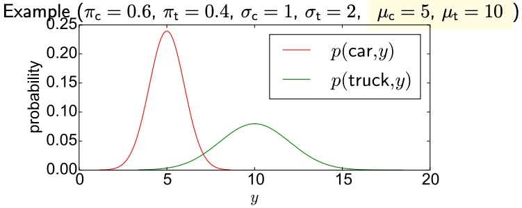
We measure lengths of vehicles. The observation space is two-dimensional, with $x$ capturing vehicle type (binary) and $y$ capturing length (Gaussian).
$p(x, y)$ $x\in$ {car, truck}, $y \in \mathbb{R}$
\[p(\text {car}, y)=\pi_{\mathrm{c}} \mathcal{N}\left(y \mid \mu_{\mathrm{c}}, \sigma_{\mathrm{c}}=1\right)=\kappa_{\mathrm{c}} \exp \left\{-\frac{1}{2}\left(y-\mu_{\mathrm{c}}\right)^{2}\right\},\left(\kappa_{\mathrm{c}}=\frac{\pi_{\mathrm{c}}}{\sqrt{2 \pi}}\right)\] \[p(\text {truck,} y)=\pi_{\mathrm{t}} \mathcal{N}\left(y \mid \mu_{\mathrm{t}}, \sigma_{\mathrm{t}}=2\right)=\kappa_{\mathrm{t}} \exp \left\{-\frac{1}{8}\left(y-\mu_{\mathrm{t}}\right)^{2}\right\},\left(\kappa_{\mathrm{t}}=\frac{\pi_{\mathrm{t}}}{\sqrt{8 \pi}}\right)\]where $\pi_c + \pi_t = 1$
例三 Complete Data (Easy case)
\(T=\{\underbrace{\left(\operatorname{car}, y_{1}^{(c)}\right),\left(\operatorname{car}, y_{2}^{(c)}\right), \ldots,\left(\operatorname{car}, y_{C}^{(c)}\right)}_{C \text { car observations }}, \underbrace{\left(\text {truck}, y_{1}^{(\mathrm{t})}\right),\left(\text {truck}, y_{2}^{(\mathrm{t})}\right), \ldots,\left(\text {truck}, y_{T}^{(\mathrm{t})}\right)}_{T \text { truck observations }}\}\)
Log-likelihood
\[\ell(\mathcal{T})=\sum_{i=1}^{N} \ln p\left(x_{i}, y_{i} \mid \mu_{\mathrm{c}}, \mu_{\mathrm{t}}\right)=C \ln \kappa_{\mathrm{c}}-\frac{1}{2} \sum_{i=1}^{C}\left(y_{i}^{(c)}-\mu_{\mathrm{c}}\right)^{2}+T \ln \kappa_{\mathrm{t}}-\frac{1}{8} \sum_{i=1}^{T}\left(y_{i}^{(\mathrm{t})}-\mu_{\mathrm{t}}\right)^{2}\]很容易用 MLE 估計 $\mu_1, \mu_2$
\[\frac{\partial \ell(\mathcal{T})}{\partial \mu_{\mathrm{c}}}=\sum_{i=1}^{C}\left(y_{i}^{(\mathrm{c})}-\mu_{\mathrm{c}}\right)=0 \quad \Rightarrow \quad \mu_{\mathrm{c}}=\frac{1}{C} \sum_{i=1}^{C} y_{i}^{(c)}\] \[\frac{\partial \ell(\mathcal{T})}{\partial \mu_{\mathrm{t}}}=\frac{1}{4} \sum_{i=1}^{T}\left(y_{i}^{(\mathrm{t})}-\mu_{\mathrm{t}}\right)=0 \quad \Rightarrow \quad \mu_{\mathrm{t}}=\frac{1}{T} \sum_{i=1}^{T} y_{i}^{(\mathrm{t})}\]直觀上很容易理解。如果 observations 已經分組,求 mean 只要做 sample 的平均即可。
以這個例子,ratio $\pi_c, \pi_t$ 不論已知或未知,都不影響結果。
例四 incomplete/hidden Data
\[\mathcal{T}=\{\left(\operatorname{car}, y_{1}^{(c)}\right), \ldots,\left(\operatorname{car}, y_{C}^{(c)}\right),\left(\text {truck}, y_{1}^{(\mathrm{t})}\right), \ldots,\left(\text {truck}, y_{T}^{(\mathrm{t})}\right), \underbrace{\left(\bullet, y_{1}^{\bullet}\right), \ldots,\left(\bullet, y_{M}^{\bullet}\right)}_{\begin{array}{l} \text { data with uknown } \\ \text { vehicle type } \end{array}}\}\] \[p\left(y^{\bullet}\right)=p\left(\text {car}, y^{\bullet}\right)+p\left(\text {truck}, y^{\bullet}\right)\]Log-likelihood
\[\ell(\mathcal{T})=\sum_{i=1}^{N} \ln p\left(x_{i}, y_{i} \mid \mu_{c}, \mu_{\mathrm{t}}\right)=\overbrace{C \ln \kappa_{\mathrm{c}}-\frac{1}{2} \sum_{i=1}^{C}\left(y_{i}^{(c)}-\mu_{\mathrm{c}}\right)^{2}+T \ln \kappa_{\mathrm{t}}-\frac{1}{8} \sum_{i=1}^{T}\left(y_{i}^{(\mathrm{t})}-\mu_{\mathrm{t}}\right)^{2}}^{\text {same term as before }} \\ +\sum_{i=1}^{M} \ln \left(\kappa_{\mathrm{c}} \exp \left\{-\frac{1}{2}\left(y_{i}^{\bullet}-\mu_{\mathrm{c}}\right)^{2}\right\}+\kappa_{\mathrm{t}} \exp \left\{-\frac{1}{8}\left(y_{i}^{\bullet}-\mu_{\mathrm{t}}\right)^{2}\right\}\right)\]不用微分也知道非常難解 MLE. 我們必須用另外的方法,就是 EM 算法。 不過我們還是微分一下,得到更多的 insights.
\[\begin{aligned} 0=\frac{\partial \ell(\mathcal{T})}{\partial \mu_{\mathrm{c}}} &=\sum_{i=1}^{C}\left(y_{\mathrm{c}}^{(\mathrm{c})}-\mu_{\mathrm{c}}\right) \\ &+ \sum_{i=1}^{M} \overbrace{\frac{\kappa_{\mathrm{c}} \exp \left\{-\frac{1}{2}\left(y_{i}^{\bullet}-\mu_{\mathrm{c}}\right)^{2}\right\}}{\kappa_{\mathrm{c}} \exp \left\{-\frac{1}{2}\left(y_{i}^{\bullet}-\mu_{\mathrm{c}}\right)^{2}\right\}+\kappa_{\mathrm{t}} \exp \left\{-\frac{1}{8}\left(y_{i}^{\bullet}-\mu_{\mathrm{t}}\right)^{2}\right\}}}^{p\left(\operatorname{car} \mid y_{i}^{\bullet}, \mu_{\mathrm{c}}, \mu_{\mathrm{t}}\right)}\left(y_{i}^{\bullet}-\mu_{\mathrm{c}}\right) \end{aligned}\] \[0=4 \frac{\partial \ell(\mathcal{T})}{\partial \mu_{\mathrm{t}}}=\sum_{i=1}^{T}\left(y_{i}^{(\mathrm{t})}-\mu_{\mathrm{t}}\right)+\sum_{i=1}^{M} p\left(\text {truck} \mid y_{i}^{\bullet}, \mu_{\mathrm{c}}, \mu_{\mathrm{t}}\right)\left(y_{i}^{\bullet}-\mu_{\mathrm{t}}\right)\]上兩式非常有物理意義。基本是 easy case 的延伸:已知分類的平均值,加上未知分類的機率平均值。一個簡單的方法是只取前面已知的部分平均,不過這不是最佳,因為丟失部分的資訊。
Missing Values, EM Approach
重新 summarize optimality conditions
\[\sum_{i=1}^{C}\left(y_{i}^{(c)}-\mu_{c}\right)+\sum_{i=1}^{M} p\left(\operatorname{car} \mid y_{i}^{\bullet}, \mu_{c}, \mu_{\mathrm{t}}\right)\left(y_{i}^{\bullet}-\mu_{\mathrm{c}}\right)=0\] \[\sum_{i=1}^{T}\left(y_{i}^{(\mathrm{t})}-\mu_{\mathrm{t}}\right)+\sum_{i=1}^{M} p\left(\text {truck } \mid y_{i}^{\bullet}, \mu_{\mathrm{c}}, \mu_{\mathrm{t}}\right)\left(y_{i}^{\bullet}-\mu_{\mathrm{t}}\right)=0\]如果 $p(\text {truck} \mid y_{i}^{\bullet}, \mu_c, \mu_t)$ 和 $p(\text {car} \mid y_{i}^{\bullet}, \mu_c, \mu_t)$ 已知,上式非常容易解 $\mu_c$ and $\mu_t$。實際這是一個雞生蛋、蛋生雞的問題,因為這兩個機率又和 $\mu_c$ and $\mu_t$ 相關。
EM algorithm 剛好用來打破這個迴圈。
- Let $z_i \,(i=1, 2, \cdots, M), z_i \in \text{{car, truck}}$ denote the missing data. Define $q\left(z_{i}\right)=p\left(z_{i} \mid y_{i}^{\bullet}, \mu_{\mathrm{c}}, \mu_{\mathrm{t}}\right)$
- 上述 optimality equations 可以得到
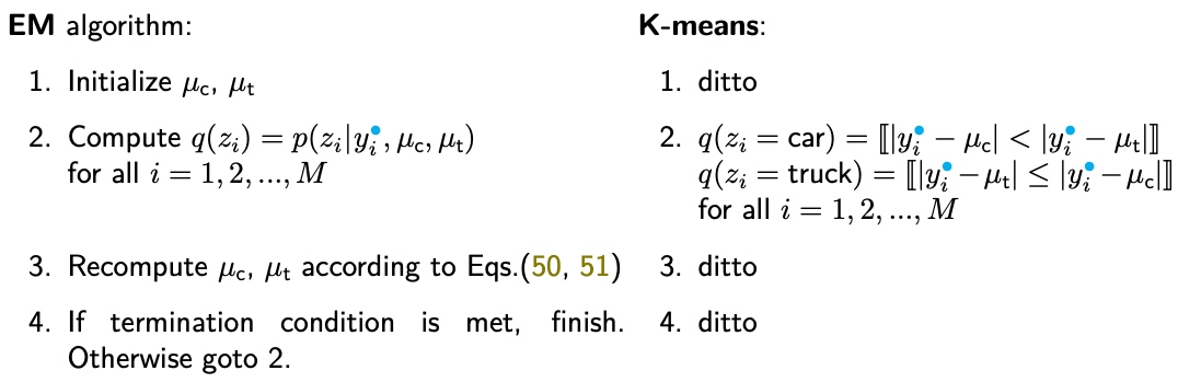
EM Algorithm 可以用以下四步驟表示
- Initialize $\mu_c$, $\mu_t$
- Compute $q\left(z_{i}\right)=p\left(z_{i} \mid y_{i}^{\bullet}, \mu_{\mathrm{c}}, \mu_{\mathrm{t}}\right)$ for $i = 1, 2, \cdots, M$
- Recompute $\mu_c$, $\mu_t$ according to the above equations.
- If termination condition is met, finish. Otherwise, goto 2.
上述步驟 2 稱為 Expectation (E) Step, 步驟 3 稱為 Maximization (M) Step. 統稱為 EM algorithm.
Q. Why Step 2 稱為 Expectation? not clear. Maximization 比較容易理解,因為 optimality condition 就是 maximization (微分為 0).
In summary, EM algorithm 的一個關鍵點是:讓 incomplete/hidden data 變成 complete (Expectation?). 有了完整的 data, 就容易用 MLE 找到 maximal likelihood estimation ($\mu_c$ and $\mu_t$ in this case).
Clustering: Soft Assignment Vs. Hard Assignment (K-means)
EM Algorithm Derivation
EM algorithm 如果只是 heuristic algorithm, 可能有用度大幅縮減。以下討論 EM 數學上的 formulation. 先定義 terminologies
- $\mathbf{x}$: observed random variables (下圖雙圓框)
- $\mathbf{z}$: hidden random variables (下圖單圓框)
- $\mathbf{\theta}$: fixed model parameters to be estimated (下圖單方框)
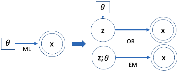
目標:Find $\theta^*$ to maximize likelihood or marginal likelihood 如下 $\eqref{eqMLE}$. 此處 $\theta$ 是一個 fixed parameter, 不是一個 random variable. 所以我們用 $p(x; \theta)$ notation, 而避免用 $p(x \mid \theta)$ notation. 不過有時候引用其他文章還是難以完全避免,可以從上下文判斷。
\[\begin{align} \boldsymbol{\theta}^{*}=\underset{\boldsymbol{\theta}}{\operatorname{argmax}} \ell(\boldsymbol{\theta})=\underset{\boldsymbol{\theta}}{\operatorname{argmax}} \ln p(\mathbf{x} ; \boldsymbol{\theta}) \label{eqMLE} \end{align}\]思路:假設解下列完整 data 很容易解 (例如例一和例三)
\[\begin{align} \underset{\boldsymbol{\theta}}{\operatorname{argmax}} \ln p(\mathbf{x}, \mathbf{z} ; \boldsymbol{\theta}) \label{eqMLE2} \end{align}\]我們的想法是把 $\eqref{eqMLE}$ 先變形成上式 $\eqref{eqMLE2}$,再想辦法優化
\[\begin{align} \ln p(\mathbf{x} ; \boldsymbol{\theta}) &=\ln \sum_{\mathbf{z}} p(\mathbf{x}, \mathbf{z} ; \boldsymbol{\theta}) \nonumber \\ &=\ln \sum_{\mathbf{z}} q(\mathbf{z}) \frac{p(\mathbf{x}, \mathbf{z} ; \boldsymbol{\theta})}{q(\mathbf{z})} \label{eqMLE3} \end{align}\]這裡引入看似任意 probability distribution $q(\mathbf{z})$ with $\sum_{\mathbf{z}} q(\mathbf{z})=1$. 後面會說明如何選 $q(\mathbf{z})$.
Log-Likelihood with Hidden Variable Lower Bound
上式 $\eqref{eqMLE3}$ 利用 Jensen’s inequality 可以導出 $\geq \sum_{\mathbf{z}} q(\mathbf{z}) \ln \frac{p(\mathbf{x}, \mathbf{z} ; \boldsymbol{\theta})}{q(\mathbf{z})}$
我們定義 $\ln p(\mathbf{x} ; \boldsymbol{\theta})$ 的 lower bound or ELBO (Evidence Lower BOund) 為 $\mathcal{L}(q, \boldsymbol{\theta})$, for any distribution $q(\mathbf{z})$.
\[\begin{align} \mathcal{L}(q, \boldsymbol{\theta})=\sum_{\mathbf{z}} q(\mathbf{z}) \ln \frac{p(\mathbf{x}, \mathbf{z} ; \boldsymbol{\theta})}{q(\mathbf{z})} \label{eqELBO} \end{align}\]這已經非常接近思路!我們的思路修正成把有 hidden data 的 MLE 變成用完整 data 的 MLE 做為 lower bound. 再通過 $q(\mathbf{z})$ 提高 lower bound 逼近原來的目標。
Maximizing $\mathcal{L}(q, \boldsymbol{\theta})$ by choosing $q(\mathbf{z})$ 就可以 push the log likelihood $\ln p(\mathbf{x} ; \boldsymbol{\theta})$ upwards.
反過來我們可以計算和 lower bound 之間的 gap.
\[\begin{align} \ln p(\mathbf{x}, \boldsymbol{\theta})-\mathcal{L}(q; \boldsymbol{\theta}) &=\ln p(\mathbf{x} ; \boldsymbol{\theta})-\sum_{\mathbf{z}} q(\mathbf{z}) \ln \frac{p(\mathbf{x}, \mathbf{z} ; \boldsymbol{\theta})}{q(\mathbf{z})} \nonumber\\ &=\ln p(\mathbf{x} ; \boldsymbol{\theta})-\sum_{\mathbf{z}} q(\mathbf{z})\{\ln \underbrace{p(\mathbf{x}, \mathbf{z} ; \boldsymbol{\theta})}_{p(\mathbf{z} \mid \mathbf{x}; \boldsymbol{\theta}) p(\mathbf{x} ; \boldsymbol{\theta})}-\ln q(\mathbf{z})\} \nonumber\\ &=\ln p(\mathbf{x} ; \boldsymbol{\theta})-\sum_{\mathbf{z}} q(\mathbf{z})\{\ln p(\mathbf{z} \mid \mathbf{x}; \boldsymbol{\theta})+\ln p(\mathbf{x} ; \boldsymbol{\theta})-\ln q(\mathbf{z})\} \nonumber\\ &=\ln p(\mathbf{x} ; \boldsymbol{\theta})-\underbrace{\sum_{\mathbf{z}} q(\mathbf{z})}_{1} \ln p(\mathbf{x} ; \boldsymbol{\theta})-\sum_{\mathbf{z}} q(\mathbf{z})\{\ln p(\mathbf{z} \mid \mathbf{x}; \boldsymbol{\theta})-\ln q(\mathbf{z})\} \nonumber\\ &=-\sum_{\mathbf{z}} q(\mathbf{z}) \ln \frac{p(\mathbf{z} \mid \mathbf{x}; \boldsymbol{\theta})}{q(\mathbf{z})} \label{eqGAP} \\ &= D_{\mathrm{KL}}(q(\mathbf{z}) \| p(\mathbf{z} \mid \mathbf{x}; \boldsymbol{\theta}) ) \ge 0 \label{eqKL} \end{align}\]這個 gap $\eqref{eqKL}$ 深具物理意義,就是 KL divergence between $q(\mathbf{z})$ and posterior $p(\mathbf{z} \mid \mathbf{x}; \boldsymbol{\theta})$, 也就是兩者之間的距離,永遠大於 0. 這也和 Jensen Inequality 的結論一致!
以下是關鍵:
- 如果能找到 $q(\mathbf{z}) = p(\mathbf{z} \mid \mathbf{x}; \boldsymbol{\theta})$ 的 analytical solution,就可以讓 gap 變成 0. Lower bound $\eqref{eqELBO}$ 就是我們要 maximize 目標,voila!
- 例如例四 GMM 的 $p(\mathbf{z} \mid \mathbf{x}; \boldsymbol{\theta})$ 就是 softmax function.
- 即使 $q(\mathbf{z})$ 有 analytical solution, e.g. softmax, 不代表容易解 maximum 以及對應的 parameter. EM algorithm 就是用來處理這個問題,見下文。
- 假如 $q(\mathbf{z})$ 非常複雜沒有 analytical solution,還有另外方法:variational approximation; 稱為 Bayesian inference;或是用一個 neural network approximate posterior;稱為 variational autoencoder (VAE). 本文不討論,下文再討論。
EM Algorithm Push the Lower Bound Upwards
Log likelihood function 可以分為兩個部分: ELBO + KL Gap of posterior
\[\begin{equation} \ln p(\mathbf{x} ; \boldsymbol{\theta})=\mathcal{L}(q, \boldsymbol{\theta})+ D_{\mathrm{KL}}(q(\mathbf{z}) \| p(\mathbf{z} \mid \mathbf{x}; \boldsymbol{\theta}) ) \end{equation}\label{eqSUM}\]從 Jensen’s inequality 得到 $\mathcal{L}(q; \boldsymbol{\theta})$ 是 lower bound. 從 KL divergence $\ge$ 0 再度驗證。
如果 $q(\mathbf{z}) = p(\mathbf{z} \mid \mathbf{x}; \boldsymbol{\theta})$, the bound is tight.
接下來看兩個極端的 examples.
Trivial Case: Hidden variable $\mathbf{z}$ does NOT provide any information of $\mathbf{x}$
如果 $\mathbf{x}$ 和 $\mathbf{z}$ 完全無關,$p(\mathbf{z} \mid \mathbf{x}; \boldsymbol{\theta}) = p(\mathbf{z} ; \boldsymbol{\theta})$. We can make $q(\mathbf{z}) = p(\mathbf{z} ; \boldsymbol{\theta})$ such that $D_{\mathrm{KL}}(q(\mathbf{z}) | p(\mathbf{z} \mid \mathbf{x}; \boldsymbol{\theta})) = 0$, 也就是 gap = 0. Lower bound 就變成原來的 log-likelihood function, trivial case.
\[\begin{aligned} \mathcal{L}(q, \boldsymbol{\theta}) &= \sum_{\mathbf{z}} q(\mathbf{z}) \ln \frac{p(\mathbf{x}, \mathbf{z} ; \boldsymbol{\theta})}{q(\mathbf{z})}\\ &= \sum_{\mathbf{z}} q(\mathbf{z}) \ln \frac{p(\mathbf{x} ; \boldsymbol{\theta}) p(\mathbf{z} ; \boldsymbol{\theta})}{q(\mathbf{z})} \\ &= \sum_{\mathbf{z}} q(\mathbf{z}) \ln p(\mathbf{x} ; \boldsymbol{\theta})\\ &= \ln p(\mathbf{x} ; \boldsymbol{\theta}) \end{aligned}\]Case 2: 如果 $p(\mathbf{z} \mid \mathbf{x}; \boldsymbol{\theta})$ 有 analytical solution, let $q(\mathbf{z}) = p(\mathbf{z} \mid \mathbf{x}; \boldsymbol{\theta})$
\[\begin{aligned} \mathcal{L}(q, \boldsymbol{\theta}) &= \sum_{\mathbf{z}} q(\mathbf{z}) \ln \frac{p(\mathbf{x}, \mathbf{z} ; \boldsymbol{\theta})}{q(\mathbf{z})}\\ &= \sum_{\mathbf{z}} q(\mathbf{z}) \ln \frac{p(\mathbf{z} \mid \mathbf{x}; \boldsymbol{\theta}) p(\mathbf{x} ; \boldsymbol{\theta})}{q(\mathbf{z})} \\ &= \sum_{\mathbf{z}} q(\mathbf{z}) \ln p(\mathbf{x} ; \boldsymbol{\theta})\\ &= \ln p(\mathbf{x} ; \boldsymbol{\theta}) \end{aligned}\]其實這就是 EM algorithm 的精髓
EM 具體步驟
Recap EM algorithm:
- Gap 可以視為從 observables 推論出 unobservables, i.e. incomplete/hidden data, 對應 EM algorithm 的 E-Step.
- Lower bound 其實可以視為 MLE of complete data, 對應 EM algorithm 的 M-Step.
Recap lower bound $\eqref{eqELBO}$ 包含兩個部分:(i) $q(\mathbf{z})$ distribution and (ii) log-likelihood of complete data, $\ln p(\mathbf{x}, \mathbf{z} ; \boldsymbol{\theta})$.
這兩個部分剛好對應 EM algorithm 的 E-step (i) and M-step (ii).
- Initialize $\boldsymbol{\theta}=\boldsymbol{\theta}^{(0)}$
- E-step (Expectation):
- M-step (Maximization):
M-step: $q^{(t+1)}$ is fixed
我們先看 M-step $\eqref{eqMstep}$, 因為這和 MLE estimate $\theta$ 非常相似。
\[\begin{aligned} \mathcal{L}\left(q^{(t+1)}, \boldsymbol{\theta}\right) &=\sum_{\mathbf{z}} q^{(t+1)}(\mathbf{z}) \ln \frac{p(\mathbf{x}, \mathbf{z} ; \boldsymbol{\theta})}{q^{(t+1)}(\mathbf{z})} \\ &=\sum_{\mathbf{z}} q^{(t+1)}(\mathbf{z}) \ln p(\mathbf{x}, \mathbf{z} ; \boldsymbol{\theta})-\underbrace{\sum_{\mathbf{z}} q^{(t+1)}(\mathbf{z}) \ln q^{(t+1)}(\mathbf{z})}_{\text {const. }} \end{aligned}\] \[\begin{align} \boldsymbol{\theta}^{(t+1)}=\underset{\boldsymbol{\theta}}{\operatorname{argmax}} \sum_{\mathbf{z}} q^{(t+1)}(\mathbf{z}) \ln p(\mathbf{x}, \mathbf{z} ; \boldsymbol{\theta}^{(t)}) \label{eqMstep2} \end{align}\]注意 M-Step 和完整 data 的 MLE 思路如下非常接近,只加了對 $q(\mathbf{z})$ 的 weighted sum. \(\underset{\boldsymbol{\theta}}{\operatorname{argmax}} \ln p(\mathbf{x}, \mathbf{z} ; \boldsymbol{\theta})\)
上式微分等於 0 就可以解 $\theta^{t+1}$。上面例四以及例二就是很好的例子。
另一個常見的寫法
\[\begin{align} \boldsymbol{\theta}^{(t+1)}=\underset{\boldsymbol{\theta}}{\operatorname{argmax}} E_{q(z)} \ln p(\mathbf{x}, \mathbf{z} ; \boldsymbol{\theta}^{(t)}) \label{eqMstep3} \end{align}\]注意 M-Step 是 maximize lower bound, 並不等於 maximize 不完整 data 的 MLE,因為還差了一個 gap function (i.e. KL divergence). E-Step 的目標才是縮小 gap function, which is also $\boldsymbol{\theta}$ dependent.
E-step: $\boldsymbol{\theta}^{(t)}$ is fixed
\[q^{(t+1)}=\underset{q}{\operatorname{argmax}} \mathcal{L}\left(q, \boldsymbol{\theta}^{(t)}\right)\] \[\mathcal{L}\left(q, \boldsymbol{\theta}^{(t)}\right)=\underbrace{\ln p\left(\mathbf{x} ; \boldsymbol{\theta}^{(t)}\right)}_{\text {const. }}-D_{\mathrm{KL}}(q \| p)\]以上 KL divergence 大於等於 0,所以 maximize lower bound 就要讓 要選擇 $q(z)$ 儘量縮小 gap (i.e. KL divergence) 到 0. Gap 等於 0 的條件就是
\[\begin{align} q^{(t+1)}(\mathbf{z}) = p(\mathbf{z} \mid \mathbf{x}; \boldsymbol{\theta}^{(t)}) \label{eqEstep2} \end{align}\]同樣 E-Step 深具物理意義,就是猜 incomplete/hidden data distribution based on 已知的 observables 和 iterative $\theta$.
例如例四 E-Step 就是計算 $q\left(z_{i}\right)=p\left(z_{i} \mid y_{i}^{\bullet}, \mu_{\mathrm{c}}, \mu_{\mathrm{t}}\right)$ for $i = 1, 2, \cdots, M$. 結果是 softmax function.
Conditional Vs. Joint Distribution
我們可以把 conditional distribution 改成 joint distribution 如下。兩者都可以用來解 E-Step.
\[p(\mathbf{z} \mid \mathbf{x}; \boldsymbol{\theta}^{(t)}) = p(\mathbf{z}, \mathbf{x} ; \boldsymbol{\theta}^{(t)}) / p(\mathbf{x} ; \boldsymbol{\theta}^{(t)})\]EM 精髓: 結合 E-Step and M-Step
如果 E-Step $\eqref{eqEstep2}$ 有 analytic solution, 可以代入 M-Step $\eqref{eqMstep2}$ 得到有名的 $Q$ function:
\[\begin{align} Q(\theta^{t+1} | \theta^{t}) &= \sum_{\mathbf{z}} p(\mathbf{z} \mid \mathbf{x}; \boldsymbol{\theta}^{(t)}) \ln p(\mathbf{x}, \mathbf{z} ; \boldsymbol{\theta}^{t+1}) \nonumber \\ &= \int d \mathbf{z} \, p(\mathbf{z} \mid \mathbf{x}; \boldsymbol{\theta}^{(t)}) \ln p(\mathbf{x}, \mathbf{z} ; \boldsymbol{\theta}^{t+1}) \\ &= E_{z\sim p(\mathbf{z} \mid \mathbf{x}; \boldsymbol{\theta}^{(t)})} \ln p(\mathbf{x}, \mathbf{z} ; \boldsymbol{\theta}^{(t+1)}) \end{align}\]New EM algorithm with fixed $\boldsymbol{\theta}^{t}$
\[\begin{align} \boldsymbol{\theta}^{(t+1)}=\underset{\boldsymbol{\theta}}{\operatorname{argmax}} Q(\boldsymbol{\theta}^{t+1} | \boldsymbol{\theta}^{t}) \label{eqQ} \end{align}\]Q&A
From $\eqref{eqELBO}$, 我們可以得到
\[\begin{align} \mathcal{L}(q, \boldsymbol{\theta})&=\sum_{\mathbf{z}} q(\mathbf{z}) \ln \frac{p(\mathbf{x}, \mathbf{z} ; \boldsymbol{\theta})}{q(\mathbf{z})} \nonumber \\ &= - D_{\mathrm{KL}}(q(\mathbf{z}) \| p(\mathbf{z}, \mathbf{x}; \boldsymbol{\theta}) ) \label{eqELBOKL} \end{align}\]代入 $\eqref{eqKL}$, 我們可以得到
\[\begin{align} \ln p(\mathbf{x}; \boldsymbol{\theta}) &= \mathcal{L}(q; \boldsymbol{\theta}) + D_{\mathrm{KL}}(q(\mathbf{z}) \| p(\mathbf{z} \mid \mathbf{x}; \boldsymbol{\theta}) ) \nonumber \\ &= - D_{\mathrm{KL}}(q(\mathbf{z}) \| p(\mathbf{z}, \mathbf{x}; \boldsymbol{\theta}) ) + D_{\mathrm{KL}}(q(\mathbf{z}) \| p(\mathbf{z} \mid \mathbf{x}; \boldsymbol{\theta}) ) \nonumber \end{align}\]也就是 ELBO = $\mathcal{L}(q; \boldsymbol{\theta}) = - D_{\mathrm{KL}}(q(\mathbf{z}) | p(\mathbf{z}, \mathbf{x}; \boldsymbol{\theta}) )$. 我們可以反過來驗證
\[\begin{align} \ln p(\mathbf{x}; \boldsymbol{\theta}) &= \sum_z q(z) \ln p(\mathbf{x}; \boldsymbol{\theta}) \nonumber \\ &= \sum_z q(z) \ln \frac{p(z, x; \theta)}{q(z)} \frac{q(z)}{p(z \mid x; \theta)} \nonumber \\ &= \sum_z q(z) \ln \frac{p(z, x; \theta)}{q(z)} + \sum q(z) \ln \frac{q(z)}{p(z \mid x; \theta)} \nonumber \\ &= - D_{\mathrm{KL}}(q(\mathbf{z}) \| p(\mathbf{z}, \mathbf{x}; \boldsymbol{\theta}) ) + D_{\mathrm{KL}}(q(\mathbf{z}) \| p(\mathbf{z} \mid \mathbf{x}; \boldsymbol{\theta}) ) \label{eqKL3} \end{align}\]$\eqref{eqKL3}$ 不免讓人浮想翩翩。 KL divergence 一定為大於等於 0.
- 如果要 maximize (marginal) likelihood $\ln p(x; \theta)$, 好像正確的做法是讓 $\eqref{eqKL3}$ maximize 第一個 KL divergence 為 0; 第二個 KL divergence 越大越好?
- e.g. let $q(z) = p(z, x; \theta) \to \ln p(x; \theta) = 0 + D_{K L}(p(z, x; \theta) | p(z \mid x; \theta) \ge 0$
- 但我們知道 $\ln p(x;\theta) < 0$, 如何解釋這個矛盾?
- 一個是 $\eqref{eqELBOKL}$ 寫成 KL divergence 有問題。因為 KL divergence 是兩個同樣 dimension distribution 的距離 measurement. $\eqref{eqELBOKL}$ 的 joint distribution $(z, x)$ 的 dimension 大於 $q(z)$,寫成 KL divergence 無意義,也沒有距離的觀念。除非把 joint distribution marginalized 成 $p(z)$, i.e. prior, 才能和 $q(z)$ 做 KL divergence. 或者 with a fixed $x=c$, $\int p(z, x=c; \theta) = 1$ 才能滿足 distribution 的定義。
- 但是 conditional distribution $p(z\mid x)$, i.e. posterior 和 $q(z)$ 則是同樣的 dimension, KL divergence 有意義。
-
實務上,我們的做法完全不同,甚至相反。正確的表示式 from $\eqref{eqKL}$ 得到:
\[\begin{align} \ln p(\mathbf{x}; \boldsymbol{\theta}) &= \sum_z q(z) \ln \frac{p(z, x; \theta)}{q(z)} + D_{\mathrm{KL}}(q(\mathbf{z}) \| p(\mathbf{z} \mid \mathbf{x}; \boldsymbol{\theta})) \end{align}\]- 我們 maximize 第一項 lower bound (ELBO), 以及 minimize 第二項 KL divergence 為 0
- e.g. $q(z) = p(z \mid x; \theta) \to \ln p(x; \theta) = E_{q(z)} \ln p(z, x; \theta) + H(q) + 0$
- 重點是 find $\theta^* = \arg \max_{\theta} E_{p(z\mid x; \theta)} \ln p(z, x; \theta)$
Free Energy Interpretation [@poczosCllusteringEM2015]
搞 machine learning 很多是物理學家 (e.g. Max Welling), 習慣用物理觀念套用於 machine learning. 常見的例子是 training 的 momentum method. 另一個是 energy/entropy loss function. 此處我們看的是類似 energy loss function.
我們從 gap 開始
\[\ln p(\mathbf{x} ; \boldsymbol{\theta})-\mathcal{L}(q, \boldsymbol{\theta}) = D_{\mathrm{KL}}(q(\mathbf{z}) \| p(\mathbf{z} \mid \mathbf{x}; \boldsymbol{\theta}) ) \ge 0\] \[\begin{aligned} \ln p(\mathbf{x} ; \boldsymbol{\theta}) &= \mathcal{L}(q, \boldsymbol{\theta}) + D_{\mathrm{KL}}(q(\mathbf{z}) \| p(\mathbf{z} \mid \mathbf{x}; \boldsymbol{\theta}) ) \\ &= \sum_{\mathbf{z}} q(\mathbf{z}) \ln \frac{p(\mathbf{x}, \mathbf{z} ; \boldsymbol{\theta})}{q(\mathbf{z})} + D_{\mathrm{KL}}(q(\mathbf{z}) \| p(\mathbf{z} \mid \mathbf{x}; \boldsymbol{\theta}) ) \\ &= \sum_{\mathbf{z}} q(\mathbf{z}) \ln p(\mathbf{x}, \mathbf{z} ; \boldsymbol{\theta}) + \sum_{\mathbf{z}} -q(\mathbf{z}) \ln {q(\mathbf{z})}+ D_{\mathrm{KL}}(q(\mathbf{z}) \| p(\mathbf{z} \mid \mathbf{x}; \boldsymbol{\theta}) ) \\ &= E_{q(z)} \ln p(\mathbf{x}, \mathbf{z} ; \boldsymbol{\theta}) + H(q) + D_{\mathrm{KL}}(q(\mathbf{z}) \| p(\mathbf{z} \mid \mathbf{x}; \boldsymbol{\theta}) ) \\ \end{aligned}\]where H(q) is the entropy of q, 第一項是負的,第二項和第三項是正的。 我們用一個例子來驗證 q = {0 or 1} with 50% chance, => H(q) = 1 (bit) or ln (?) > 0 Eq(z) ln p(o, z) = -(0.5 (o-u1)^2 + 0.5 (o-u2)^2 ) / sqrt(2pi) < 0
此處我們 switch to [@poczosCllusteringEM2015] notation.
- Observed data: $D = {x_1, \cdots, x_n}$
- Unobserved/hidden variable: $z = {z_1, \cdots, z_n}$
- Parameter: $\theta = [\mu_1, \cdots, \mu_K, \pi_1, \cdots, \pi_K, \Sigma_1, \cdots, \Sigma_K]$
- Goal: $\boldsymbol{\theta}^{*}=\underset{\boldsymbol{\theta}}{\operatorname{argmax}} \ln p(D \mid \theta)$
重寫上式:
\[\begin{aligned} \ln p(D ; \boldsymbol{\theta}^t) &= \sum_{\mathbf{z}} q(\mathbf{z}) \ln p(D, \mathbf{z} ; \boldsymbol{\theta}^t) + \sum_{\mathbf{z}} -q(\mathbf{z}) \ln {q(\mathbf{z})}+ D_{\mathrm{KL}}(q(\mathbf{z}) \| p(\mathbf{z} \mid D; \boldsymbol{\theta}^t) ) \\ &= E_{q(z)} \ln p(D, \mathbf{z} ; \boldsymbol{\theta}) + H(q) + D_{\mathrm{KL}}(q(\mathbf{z}) \| p(\mathbf{z} \mid D; \boldsymbol{\theta}^t) ) \\ &= F_{\theta^t} (q(\cdot), D) + D_{\mathrm{KL}}(q(\mathbf{z}) \| p(\mathbf{z} \mid D; \boldsymbol{\theta}) ) \end{aligned}\]$F_{\theta^t} (q(\cdot), D)$ 稱為 free energy (也就是 ELBO), 包含 joint distribution expectation 和 self-entropy.
如果 $p(z\mid x; \theta)$ is analytically available (e.g. GMM, this is just a softmax!). The E-step 基本就是代入 $p(z\mid x; \theta)$ 到 LBO becomes a Q(theta, theta^old) function + H(q)
The EM algorithm can be summzied as argmax Q!!
-
E-step: 代入 $p(z\mid D)$ 到 free-energy (ELBO) update Q function (忽略 self-entropy)
- \[Q\left(\theta \mid \theta^{t}\right)=\int d y P\left(y \mid D, \theta^{t}\right) \log P(y, D \mid \theta)\]
-
M-step; argmax Q
- \[\theta^{t+1}=\arg \max _{\theta} Q\left(\theta \mid \theta^{t}\right)\]
It can be proved
-
log likelihood is always increasing! i.e. $\ln P(D\mid \theta^t) \le \ln P(D\mid \theta^{t+1})$ 這是 EM 的重要特徵!
-
Use multiple, randomized initialization in practice to avoid strucking at local minima.
Variational Expectation Maximization
EM algorithm 一個問題是對於複雜的問題沒有 analytical from $p(z\mid x)$, then (1) variational EM; or (2) use neural network such as variational autoencoder (VAE).
Variational EM 的重點是不用 Q function, 因為沒有 $p(z\mid x)$. 重點變成 minimize KL gap function for E-step.
-
Variational E-step: Fix $\theta^t$
- \[q^{t}(\cdot)=\arg \max _{q(\cdot)} F_{\theta^{t}}(q(\cdot), D)=\underset{q(\cdot)}{\arg \min } K L\left(q(y) \| P\left(y \mid D, \theta^{t}\right)\right)\]
- 但並不保證會找到 best max/min $q(y) = p(y \mid D, \theta^t)$
-
Variational M-step; Fix $q^t$
- \[\theta^{t+1}=\arg \max _{\theta} F_{\theta}\left(q^{t}(\cdot), D\right)\]
- Variational EM 並不保證 marginal likelihood 每次都遞增!
- 關鍵問題是如何找到 $q(z)$, 下文會討論。
Appendix
例二的 Conditional Vs. Joint Distribution 解法
我們之前的 E-Step 是猜 joint distribution, $p(t, s | a, b)$.
| $s_0$ | $s_1$ | |
|---|---|---|
| $t_0$ | a | 5a |
| $t_1$ | 3b | b |
如果用上述的 conditional distribution 可以細膩的看每一個 data.
-
對於所有 $(\bullet, s_0)$ \(q(t \mid s_0, a, b)=\left\{\begin{array}{l} q\left(t_{0}\right)=p\left(t_{0} \mid s_{0}, a, b\right)=\frac{a}{a+3 b} \\ q\left(t_{1}\right)=p\left(t_{1} \mid s_{0}, a, b\right)=\frac{3 b}{a+3 b} \end{array}\right.\)
-
對於所有 $(\bullet, s_1)$ \(q(t \mid s_1, a, b)=\left\{\begin{array}{l} q\left(t_{0}\right)=p\left(t_{0} \mid s_{1}, a, b\right)=\frac{5a}{5 a+ b} \\ q\left(t_{1}\right)=p\left(t_{1} \mid s_{1}, a, b\right)=\frac{b}{5 a+ b} \end{array}\right.\)
-
對於所有 $(t_0, \bullet)$ \(q(s \mid t_0, a, b)=\left\{\begin{array}{l} q\left(s_{0}\right)=p\left(s_{0} \mid t_{0}, a, b\right)=\frac{1}{6} \\ q\left(s_{1}\right)=p\left(s_{1} \mid t_{0}, a, b\right)=\frac{5}{6} \end{array}\right.\)
-
對於所有 $(t_1, \bullet)$ \(q(s \mid t_1, a, b)=\left\{\begin{array}{l} q\left(s_{0}\right)=p\left(s_{0} \mid t_{1}, a, b\right)=\frac{3}{4} \\ q\left(s_{1}\right)=p\left(s_{1} \mid t_{1}, a, b\right)=\frac{1}{4} \end{array}\right.\)
再來是例二的 M-Step
最後再把所有 dataset 的 weighted sum $(t_i, s_j)$ 統計出來,例如 $S_0$ 個 $(\bullet, s_0) \to \frac{a}{a+3b}S_0$ 個 $(t_0, s_0)$ 和 $\frac{3b}{a+3b}S_0$ 個 $(t_1, s_0)$ $S_1$ 個 $(\bullet, s_1) \to \frac{5a}{5a+b}S_1$ 個 $(t_0, s_1)$ 和 $\frac{b}{5a+b}S_1$ 個 $(t_1, s_1)$ $T_0$ 個 $(t_0, \bullet) \to \frac{1}{6}T_0$ 個 $(t_0, s_0)$ 和 $\frac{5}{6}T_0$ 個 $(t_0, s_1)$ $T_1$ 個 $(t_1, \bullet) \to \frac{3}{4}T_1$ 個 $(t_1, s_0)$ 和 $\frac{1}{4}T_1$ 個 $(t_1, s_1)$
$(t_0, s_0)$ 個數 $\to N_{00} = \frac{1}{6}T_0+\frac{a}{a+3b}S_0$ $(t_0, s_1)$ 個數 $\to N_{01} = \frac{5}{6}T_0+\frac{5a}{5a+b}S_1$ $(t_1, s_0)$ 個數 $\to N_{10} = \frac{3}{4}T_1+\frac{3b}{a+3b}S_0$ $(t_1, s_1)$ 個數 $\to N_{11} = \frac{1}{4}T_1+\frac{b}{5a+b}S_1$
因此可以使用完整 data 的 MLE estimation: \(a'=\frac{N_{00}+N_{01}}{6 N} \quad b'=\frac{N_{10}+N_{11}}{4 N}\)