Math AI - Variational Autoencoder Vs. Variational EM Algorithm

Main Reference

• [@kingmaIntroductionVariational2019] : excellent reference
• [@escuderoVariationalAutoEncoders2020] : very good article

重點 outline

1. VAE 第一個 innovation (encoder+decoder): 使用 encoder neural network ($\phi$) 和 decoder neural network ($\theta$) 架構。從 autoencoder 的延伸似乎很直觀。但從 deterministic 延伸到 probabilistic 有點魔幻寫實，需要更嚴謹的數學框架。
2. VAE 第二個 innovation (DLVM): 引入 hidden (random) variable $\mathbf{z}$, 從 $\mathbf{z} \to \text{neural network}\,(\theta) \to \mathbf{x}.$ Hidden variable $\mathbf{z}$ 源自 (variational) EM + DAG; 再用 (deterministic) neural network of $\theta$ for parameter optimization. 這就是 DLVM (Deep Learning Variable Model) 的精神。 根據 (variational) EM:
   • E-step: 找到 $q(\mathbf{z}) \approx p_{\theta}(\mathbf{z} \mid \mathbf{x})$, 也就是 posterior, 但我們知道在 DLVM posterior 是 intractable，必須用近似
   • M-step: optimize $\theta$ based on posterior: $\underset{\boldsymbol{\theta}}{\operatorname{argmax}} E_{q(\mathbf{z})} \ln p_{\theta}(\mathbf{x}, \mathbf{z})$, 其中的 joint distribution 是 tractable, 但是 $q(\mathbf{z})$ intractable, 所以是卡在 posterior intractable 這個問題！
   • Iterate E-step and M-step in (variational EM); 在 DLVM 就變成 SGD optimization!
3. VAE 第三個 innovation 就是為了解決2.的 posterior 問題 $q(\mathbf{z}) \to q_{\phi}(\mathbf{z}\mid x)$: 用另一個 (tractable) encoder neural network $\phi$, 來近似 (intractable) posterior $q_{\phi}(\mathbf{z}\mid x) \approx p(\mathbf{z}\mid x)$
   • 因此 VAE 和 DLVM (or variational EM) 的差別在於 VAE 多了 encoder neural network $\phi$ ，所以三者的數學框架非常相似！
   • VAE 的 training loss 包含 reconstruction loss (源自 encoder+decoder) + 上面的 M-step loss (源自 variational EM)
   • Maximum likelihood optimization ~ minimum cross-entropy loss (not in this case) ~ M-step loss (in this case)
4. 同樣的方法應該可以用在很多 DLVM 應用中。如果有 intractable posterior, 就用 (encoder) neural network 近似。但問題是要有方法 train 這個 encoder. VAE 很巧妙的同時 train encoder + decoder 是用原始的 image and generative image. 需要再檢驗。

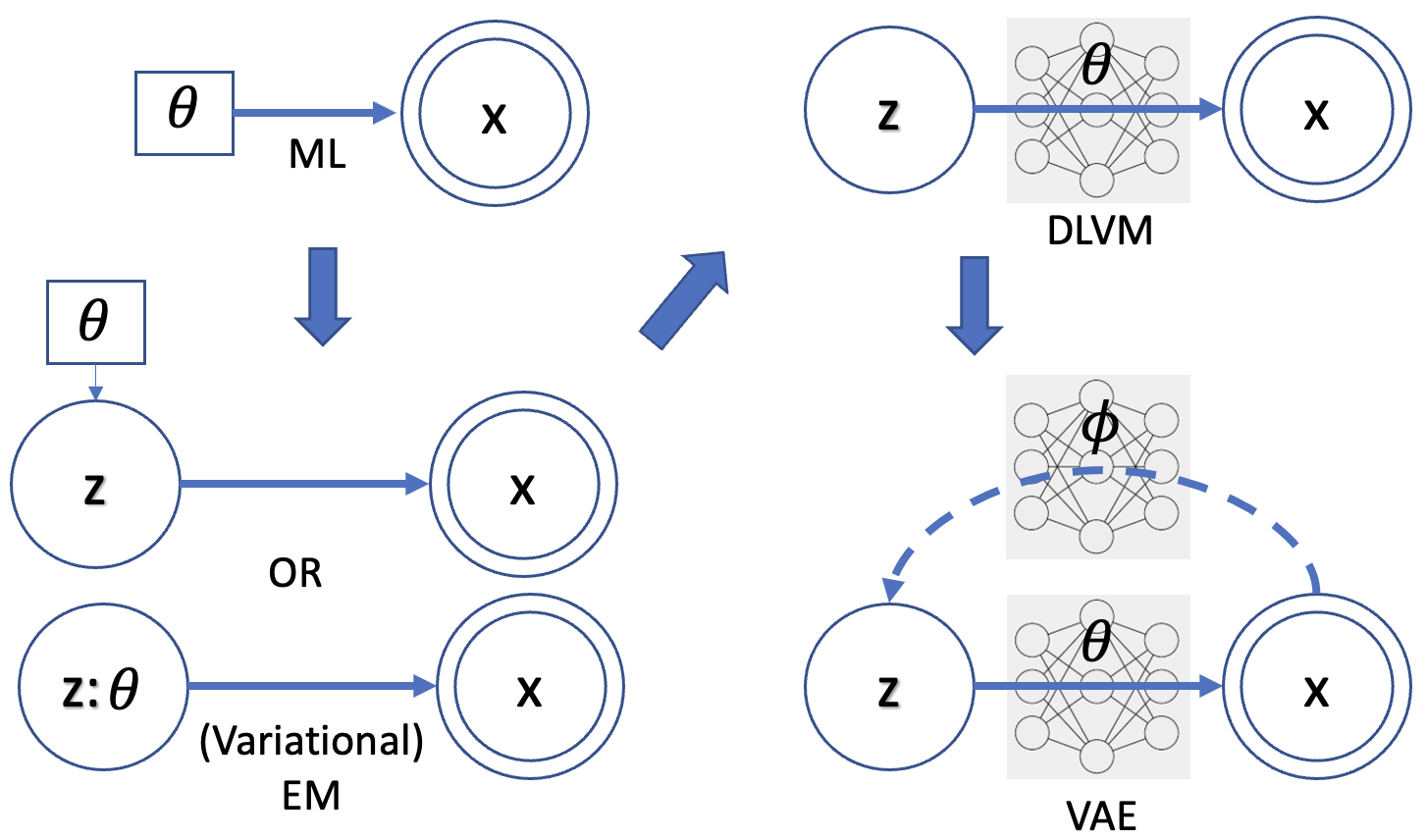
下圖顯示 ML, EM, DLVM, VAE 的演進關係；DLVM 和 VAE echo 1-4. 雙圓框代表 observed random variable, 單圓框代表 hidden random variable. 單方框代表 (fixed and to be estimated) parameter.

其他的重點：

• 如何用 deterministic neural network 表示 probabilistic bayesian inference?

• 如何用 deterministic neural network 表示 probabilistic VAE encoder and decoder?

• 如何把 intractable posterior 用 tractable neural network encoder 近似?

Variational Autoencoder, Again

第 N 次討論 VAE (variational autoencoder). 之前從 AE (autoencoder) 出發，有一些手感。但用 deterministic autoencoder 延伸想像力到 probabilistic VAE 還是隔了一層紗山。有點像二十世紀初把古典力學加上一點量子想像 ($E = h\nu$) 得到氫原子的量子光譜。雖然結果對了，但只能用在特定的情況。

或是從 “variational inference” 的出發, 掉入一堆數學中沒有抓到重點。

我們這次從 gaph+variational inference 出發。引入 neural network 變成 deep learning variable model (DLVM)。再引入 encoder neural network for posterior. 另外我們會比較 variational EM 和 VAE 增加理解。

ML estimation 和 Bayesian inference 到底有什麼差別？

簡單說 ML estimation 把 unknown/hidden 視為 a “fixed parameter” (上圖左上). Bayesian inference 把 unknown/hidden 視為 “distribution” described by a random variable (上圖左下).

有時候我們也把 $p(x;\theta)$ 寫成 conditional distribution 形式 $p(x\mid\theta).$​ 嚴格來說並不對。不過可以視為 Bayesian 詮釋的擴展。

ML estimation 做法是微分上式，解 $\theta$ parameter.

Bayesian 的觀念是: (1) $\theta$ 視為 hidden random variable; (2) 引入 hidden random variable $\mathbf{z}$ with $\theta$ as a parameter.

我們假設 (1), 利用 Bayes formula

\[p(\theta | x) = \frac{p(x | \theta) p(\theta)}{p(x)}\]

or

\[p(z | x; \theta ) = \frac{p(x | z; \theta) p(z; \theta)}{p(x)}\]

or

\[p_{\theta}(z | x) = \frac{p_{\theta}(x | z) p_{\theta}(z)}{p(x)}\]

上式的術語和解讀

• Random variable $x$ : post (事後) observations, (post) evidence. $p(x)$ 稱為 evidence distribution or marginal likelihood.
• Random variable $\mathbf{z}$ : 相對於 $x$, $\mathbf{z}$ 是 prior (事前, 先驗) 並且是 hidden variable (i.e. not evidence). 擴展我們在 maximum likelihood 的定義，從 parameter 變成 random variable. $p(z)$​​ 稱為 prior distribution.
  • 注意 prior 是 distribution, 不會出現在 ML, 因為 $z$​ 在 ML 是 parameter. 只有在 Bayesian 才有 prior (distribution)!
• Conditional distribution $p(x\mid z)$ : likelihood (或然率)。擴展我們在 maximum likelihood 的定義，從 parameter dependent distribution or function 變成 conditional distribution.
• Conditional distribution $p(z\mid x)$ ： posterior, 事後機率。就是我們想要求解的東西。
  • 注意 posterior 是 conditional distribution. 有人會以為 $p(z)$ 是 prior distribution, $p(x)$​ 是 posterior distribution. Wrong!
  • Posterior 不會出現在 ML, 只有在 Bayesian 才會討論 posterior (distribution)!
• 簡言之：Posterior $\propto$ Likelihood x Prior $\to p(z \mid x) \propto {p(x \mid z) \times p(z)}$

  • 一般我們忽略 $p(x)$ ，因為它和要 estimate 的 $z$​​ distribution (or parameter) 無關，視為常數忽略。

  • 很好記: 事後 = 事前 x 喜歡 (likelihood). 如果很喜歡，才會有事後。如果不喜歡，事後不理 (0分)

  • Prior 和 posterior (事前/先驗，事後) 都是 Bayesian 才有的說法。 ML (or Frequentist) 不會有 prior and posterior 說法。

  • 以通信為例，$z$ 是 transmitted signal (unknown), $x$ 是 received signal, $x = z + n$, 是 transmitted signal 加 noise. 如果只根據 $p(\text{received signal}\mid\text{transmitted signal}) = p(x\mid z)$

Bayesian Inference for VAE 思路

我們的問題比較類似 (2), 引入一個 hidden variable, z, with parameter $\theta$. 這和 EM algorithm 的想法完全一樣。藉著引入 hidden variable to account for some incomplete information (參考 EM article of incomplete data).

一般 Bayesian inference 是求 posterior $p(z\mid x; \theta)$, or maximize the likelihood $p(x \mid z; \theta)$. 我們待會談到 VAE，卻是要找 $p(x)$, i.e. marginal likelihood. 數學上是 $p(x) = \int_{z} p(x, z; \theta) dz = \int_{z} p(x \mid z; \theta)p(z) dz $; where $\theta$ 是 parameter, not a random variable.

另一個表示式 $p(x)= \int_{z} p(z \mid x)p(x) dx$ 顯然不行，因為 $p(x)$ 就是我們要找的 unknown.

所以我們現在缺 likelihood $p(x\mid z)$ and prior $p(z)$. $p(z)$ 不是問題，基本就是假設。會隨著 more evidence x 而被取代。我們在 VAE 一般用 N(0, 1). 理論上可以用其他的 distribution, but why bother. 現在問題就是如何求 posterior $p(x\mid z)$. 結論就是用 VAE 來 train 一個 $p(x\mid z)$.

Deterministic Neural Network Vs. Probabilistic Bayesian Inference, How?

對於 random variable 如 $x$ or $z$, 總有兩個截然不同的面向：(1) (deterministic) distribution function, $p(x), p(z)$; 以及 (2) random sample $\mathbf{x} = {x_1, x_2, \cdots, x_k}$, $\mathbf{z} = {z_1, z_2, \cdots, z_k}.$ 一般常用 deterministic function maps random samples $z_i = f(x_i)$ from $x$ space to $z$ space. 因此 $p(x)$ distribution 可以轉換成 $p(z)$ distribution. 實務上我們常常用 function 把一個 distribution 轉成另一個 distribution, 例如 uniform distribution to normal distribution. Neural network 其實就是一個比較複雜的 (deterministic) function. 這部分沒有問題。

問題是 Bayesian 需要 conditional distribution. 如果 $z = f(x)$ 是一個 deterministic neural network (or any deterministic function). 在這種情況下，conditional probability $p(z\mid x)$ 在 given $x$ 時, $z$ 卻是一個定值 ，無法變成 distribution (or a delta distribution)? 因為每一個 $x$ 只對應一個 $z$, 沒有所謂 distribution.

因此如何讓 deterministic neural network 用於 Bayesian inference? 有以下幾種可能性：

Example 1：Two neural networks from a hidden random variable to create conditional distribution. Only for demonstration, not use here

Deterministic functions 可以產生 conditional probability. 如下例

https://en.wikipedia.org/wiki/Conditional_probability_distribution

Consider the roll of a fair die and let $X=1$ if the number is even (i.e. 2, 4, or 6) and $X=0$ otherwise. Furthermore, let $Y=1$ if the number is prime (i.e. 2, 3, or 5) and $Y=0$ otherwise.

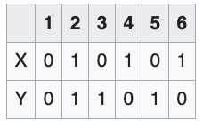
Then the unconditional probability that $X=1$ is 3/6 = 1/2 (since there are six possible rolls of the die, of which three are even), whereas the probability that $X=1$ conditional on $Y=1$ is 1/3 (since there are three possible prime number rolls—2, 3, and 5—of which one is even).

$X = f_1(Z)$ and $Y=f_2(Z)$ $Z$ 是 die 的 output random variable $1,2,\cdots,6$ 雖然 $f_1$ and $f_2$ 都是 deterministic function, 但是 $P(Y\mid X)$ 的確是 distribution, 因為我們不知道 $X=1$ 到底對應 $Z=?$

所以如果我們有一個 $Z$ random variable, 以及不同的 neural network $X = f_1(Z)$ and $Y = f_2(Z)$. Then $p(Y\mid X)$ 可以是一個 distribution 而非單一 value.

Example 2: Given Input 經過 Deterministic NN 轉成 Probabilistic Conditional Distribution

[@kingmaIntroductionVariational2019]

一般的 differentiable feed-forward neural networks are a particularly flexible and computationally scalable type of function approximator.

A particularly interesting application is probabilistic models, i.e. the use of neural networks for probability density functions (PDFs) or probability mass functions (PMFs) in probabilistic models (how?). Probabilistic models based on neural networks are computationally scalable since they allow for stochastic gradient-based optimization.

We will denote a deep NN as a vector function: NeuraNet(.). In case of neural entwork based image classifcation, for example, nerual networks parameterize a categorical distrbution $p_{\theta}(y\mid \mathbf{x})$ over a class label $y$, conditioned on an image $\mathbf{x}$. ??? y is a single label or distribution?

\[\begin{aligned} \mathbf{p} &=\operatorname{NeuralNet}_{\boldsymbol{\theta}}(\mathbf{x}) \\ p_{\boldsymbol{\theta}}(y \mid \mathbf{x}) &=\text { Categorical }(y ; \mathbf{p}) \end{aligned}\]

where the last operation of NeuralNet(.) is typical a softmax() function! such that $\Sigma_i p_i = 1$

這是很有趣的觀點。 $\mathbf{x}$ and $\mathbf{p}$ 都是 deterministic, 甚至 softmax function 都是 deterministic. 但我們賦予最後的 $y$ probabilistic distribution 涵義！基本上 NN 分類網路都是如此 (e.g. VGG, ResNet, MobileNet)。

例如 $\mathbf{x}$ 可能是一張狗照片， $\mathbf{p}$ 是 feature extraction of $\mathbf{x}$. 兩者都是 deterministic. 但最後 categorical function 直接把 $\mathbf{p}$ 賦予多值的 (deterministic) distribution, 例如狗的機率 $p_1 = 0.8,$ 貓的機率 $p_2 = 0.15,$ 其他的機率 $p_3 = 0.05.$ 這和我們一般想像的機率性 outcome, 同一個 $\mathbf{p}$ 有時 output 狗，有時 output 貓不同。

數學上這只是 vector to vector conversion, $\mathbf{p}$ 是 high dimension feature vector (e.g. 1024x1), $\mathbf{y} = [y_1, y_2, \cdots]$ 是 low dimension output vector (e.g. 3x1 or 10x1) summing to 1. 重點是這個 low dimension vector $\mathbf{y}$ 就是 conditional distribution! 也就是一個 sample $\mathbf{x}$ 就可以 output 一個 conditional distribution, 而不需要很多 $\mathbf{x}$ samples 產生 conditional distribution! 這很像量子力學中一個電子就可以產生 wave distribution, 有點違反直覺。

這似乎是把一個 random sample 轉換成一個 (deterministic) conditional distribution 的方式。不過是否是 general method, TBC.

另外這裡的 $\theta$ 就是 neural network 的 weights, determinstic parameters to be optimzed.

Neural Network and DAG (Directed Acyclic Graph)

我們 focus on directed probabilistic graphical models (PGM) or Bayesian networks. \(p_{\boldsymbol{\theta}}\left(\mathbf{x}_{1}, \ldots, \mathbf{x}_{M}\right)=\prod_{j=1}^{M} p_{\boldsymbol{\theta}}\left(\mathbf{x}_{j} \mid P a\left(\mathbf{x}_{j}\right)\right)\) where Pa(xj) is the set of parent variables of node j in the directed graph.

Traditionally, each conditional probability distribution xx is parameterized as a lookup table or a linear model.

A more flexible way to parameterize such conditional distributions is with neural networks.

\[\begin{aligned} \boldsymbol{\eta} &=\operatorname{NeuralNet}(P a(\mathbf{x})) \\ p_{\boldsymbol{\theta}}(\mathbf{x} \mid P a(\mathbf{x})) &=p_{\boldsymbol{\theta}}(\mathbf{x} \mid \boldsymbol{\eta}) \end{aligned}\]

同樣這裡的 $\theta$ 就是 neural network 的 weights, determinstic parameters to be optimzed.

重要！我們用 $\theta$ 代表這個 neural network. 這個 $\theta$ neural network 的方向是從 hidden variable $Pa(\mathbf{x})$ 到 observations $\mathbf{x}$.

Deep (Learning) Latent Variable Model (DLVM) Tractable and Intractable

以下我們用 hand-waving 方法說明幾個

\[p_{\boldsymbol{\theta}}(\mathbf{x})=\int p_{\boldsymbol{\theta}}(\mathbf{x}, \mathbf{z}) d \mathbf{z}\]

The above equation is the marginal likelihood or the model evidence, when taken as a function of $\theta$

$\theta$ 代表這個 neural network. 這個 $\theta$ neural network 的方向是從 hidden variable $\mathbf{z}$ 到 observations $\mathbf{x}$.

$p_{\boldsymbol{\theta}}(\mathbf{x}, \mathbf{z})$ : joint distribution is tractable because it includes both evidence and latent

$p_{\boldsymbol{\theta}}(\mathbf{x})$ : marginal likelihood is intractable in DLVM; 因此上式的積分也是 intractable

\[p_{\boldsymbol{\theta}}(\mathbf{x}, \mathbf{z})=p_{\boldsymbol{\theta}}(\mathbf{z}) p_{\boldsymbol{\theta}}(\mathbf{x} \mid \mathbf{z})\]

$p_{\boldsymbol{\theta}}(\mathbf{z})$ and $p_{\boldsymbol{\theta}}(\mathbf{x} \mid \mathbf{z})$ : prior and likelihood 一般 tractable because the joint distribution is tractable. 一般 prior 和 likelihood 是 tractable.

$p_{\boldsymbol{\theta}}(\mathbf{z}\mid \mathbf{x})$: posterior is intractable in DLVM because marginal likelihood is intractable

\[p_{\boldsymbol{\theta}}(\mathbf{z} \mid \mathbf{x})=\frac{p_{\boldsymbol{\theta}}(\mathbf{x}, \mathbf{z})}{p_{\boldsymbol{\theta}}(\mathbf{x})}\]

In summary

• Joint distribution, prior, likelihood 通常是 tractable, 甚至有 analytic solution.
• Marginal likelihood, posterior 通常是 intractable, 需要解但只有 approximate solution.
  • Posterior $p(z\mid x)$ => discriminative problem! given high dimension x to get a low dimension z, or $\theta$
  • Marginal likelihood p(x) => generative problem! generate a high dimension x; or sometimes given a low dimension z to generate dimensional x (conditional generative model)

以下是一個例子。

Example 3: Multivariate Bernoulli data (3 產生 conditional distribution 的方法和 2 一樣)

一個簡單的例子說明 hand-waving 的 assertion for the DLVM.

Prior $p(z)$ 是簡單的 normal distribution. Neural network 把 random sample $z$ 轉換成 $\mathbf{p}$, 再來 $\mathbf{p}$ 直接變成 Bernoulli distribution! 就像例三的 softmax 一樣。

Likelihood $\log p(x\mid z)$ 因此也是簡單的 cross-entropy, i.e. maximum likelihood ~ minimum cross-entropy loss

\[\begin{aligned} p(\mathbf{z}) &=\mathcal{N}(\mathbf{z} ; 0, \mathbf{I}) \\ \mathbf{p} &=\text { DecoderNeuralNet }_{\boldsymbol{\theta}}(\mathbf{z}) \\ \log p(\mathbf{x} \mid \mathbf{z}) &=\sum_{j=1}^{D} \log p\left(x_{j} \mid \mathbf{z}\right)=\sum_{j=1}^{D} \log \operatorname{Bernoulli}\left(x_{j} ; p_{j}\right) \\ &=\sum_{j=1}^{D} x_{j} \log p_{j}+\left(1-x_{j}\right) \log \left(1-p_{j}\right) \end{aligned}\]

where $\forall p_j \in \mathbf{p}: 0 \le p_j \le 1$

Joint distribution $p_{\boldsymbol{\theta}}(\mathbf{x}, \mathbf{z})=p_{\boldsymbol{\theta}}(\mathbf{z}) p_{\boldsymbol{\theta}}(\mathbf{x} \mid \mathbf{z})$​ 就是把兩者乘積。雖然看起來 messy, 還夾著 neural network, 但理論上 straightforward, 甚至可以寫出 analytical form.

但反過來: posterior $p(z\mid x)$, marginal likelihood $p(x)$ 即使在這麼簡單的 network, 都是難啃的骨頭！

VAE and DLVM

前面提到 基本就是把 intractable posterior inference and learning problem.

Marginal likelihood, posterior 通常是 intractable, 需要解但只有 approximate solution.

• Posterior $p(z\mid x)$ => discriminative problem! given high dimension x to get a low dimension z
• Marginal likelihood p(x) => generative problem! generate a high dimension x; or sometimes given a low dimension z to generate dimensional x (conditional generative model)

首先 target posterior $p_{\theta}(\mathbf{z}\mid \mathbf{x})$ : 注意，此處 $\theta$ 代表的 neural network (weights) from $\mathbf{z}$ to $\mathbf{x}$.

引入 encoder neural network $q_{\phi}(\mathbf{z}\mid x)$：注意，此處 $\phi$ 代表 neural network from $\mathbf{x}$ to $\mathbf{z}$.

我們希望 optimize the variational parameter $\phi$ such that

\[q_{\boldsymbol{\phi}}(\mathbf{z} \mid \mathbf{x}) \approx p_{\boldsymbol{\theta}}(\mathbf{z} \mid \mathbf{x})\]

就是讓 (tractable) encoder 近似 (intractable) posterior.

現在問題是：這個 neural network 長得怎麼樣？以及如何把 deterministic neural network 轉換成 probabilistic distribution?

Example 4：Given Input 經過 Deterministic NN 轉成 Parameters of A Random Variable to Create Conditional Distribution (e.g. VAE encoder)

Example 2 and 3 NN 產生 conditional distribution 的方式只能用在 discrete distribution. 對於 continuous distribution, NN 無法產生無限長的 distribution! 例如 VAE 使用 Normal distribution 如下：

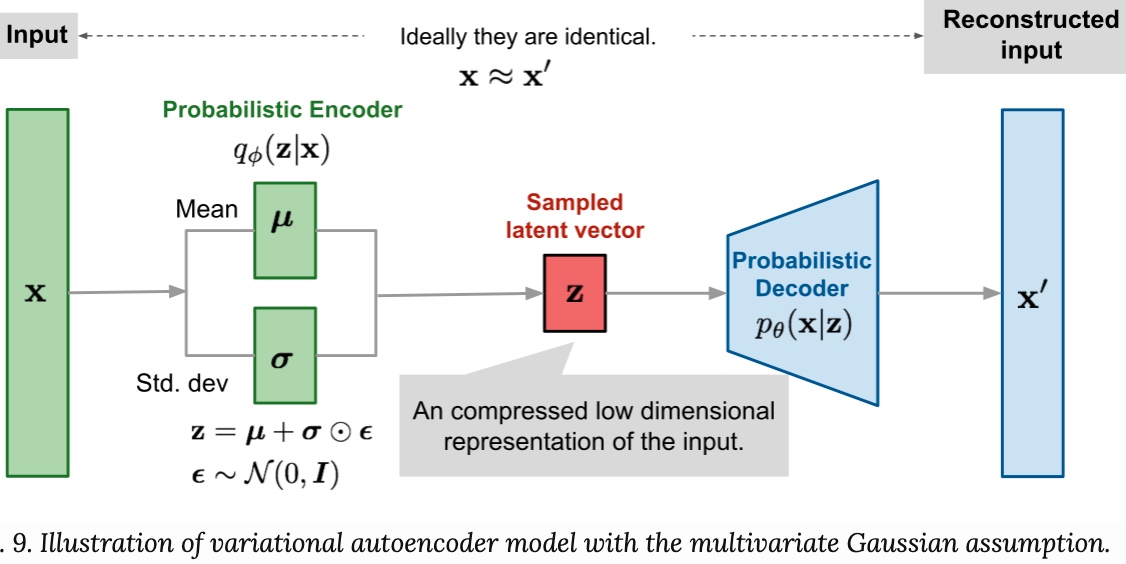
\[\begin{aligned} (\boldsymbol{\mu}, \log \boldsymbol{\sigma}) &=\text { EncoderNeuralNet }_{\boldsymbol{\phi}}(\mathbf{x}) \\ q_{\boldsymbol{\phi}}(\mathbf{z} \mid \mathbf{x}) &=\mathcal{N}(\mathbf{z} ; \boldsymbol{\mu}, \operatorname{diag}(\boldsymbol{\sigma})) \end{aligned}\]

Neural network 產生 $\mu, \log \sigma$ for normal distribution. 雖然這解決 deterministic to probabilistic 問題。但聽起來還是有點魔幻寫實方式把 deterministic to probabilistic. 這是 VAE 的實際做法。

雖然的確產生 conditional distribtuion, 但似乎比直接產生 distribution 更不直觀！例如為什麼是 $\log \sigma$, 不是 $\sigma$ 或 $1/\sigma$ ? 另外只產生 $\mu, \log \sigma$ 兩個 parameters, 是否太簡化？ 比起 softmax distribution 可能包含 10-100 parameters.

Before we can answer this question, let me quote below and move on to algorithm.

Typically, we use a single encoder neural network to perform posterior inference over all of the datapoints in our dataset. This can be contrasted to more traditional variational inference methods where the variational parameters are not shared, but instead separately and iteratively optimized per datapoint. The strategy used in VAEs of sharing variational parameters across datapoints is also called amortized variational inference (Gershman and Goodman, 2014). With amortized inference we can avoid a per-datapoint optimization loop, and leverage the efficiency of SGD.

Example 5: Decoder: How to explain $p(x\mid z)$ 的 conditional distribution?

https://towardsdatascience.com/understanding-variational-autoencoders-vaes-f70510919f73

Let’s now make the assumption that p(z) is a standard Gaussian distribution and that $p(x\mid z)$ is a Gaussian distribution whose mean is defined by a deterministic function f of the variable of z and whose covariance matrix has the form of a positive constant c that multiplies the identity matrix I. The function f is assumed to belong to a family of functions denoted F that is left unspecified for the moment and that will be chosen later. Thus, we have (不是很 make sense!)

\[\begin{aligned}(\boldsymbol{f(z)}) &=\text { DecoderNeuralNet }_{\boldsymbol{\theta}}(\mathbf{z}) \\p_{\boldsymbol{\theta}}(\mathbf{x} \mid \mathbf{z}) &=\mathcal{N}(\mathbf{x} ; \boldsymbol{f(z)}, c)\end{aligned}\] \[\begin{aligned} &p(z) \equiv \mathcal{N}(0, I) \\ &p(x \mid z) \equiv \mathcal{N}(f(z), c I) \quad f \in F \quad c>0 \end{aligned}\]

What is $c$? 似乎只能 heuristically 解釋，沒有很 solid math fondation.

一個 random generator 不夠解釋 encoder and decoder？ 那就兩個

我再想了一下，其實這可以視為 $z$ 的定義問題。我們借用 reparameterization trick 的 encoder formulation for $z$ 如下：

\[\begin{aligned}\boldsymbol{\epsilon} & \sim \mathcal{N}(0, \mathbf{I}) \\(\boldsymbol{\mu}, \log \boldsymbol{\sigma}) &=\text { EncoderNeuralNet }_{\phi}(\mathbf{x}) \\\mathbf{z} &=\boldsymbol{\mu}+\boldsymbol{\sigma} \odot \boldsymbol{\epsilon}\end{aligned}\]

我們可以分解 $\boldsymbol{\epsilon} = \boldsymbol{\epsilon}_1 + \boldsymbol{\epsilon}_2$ 都是 random variables.

\[\begin{aligned} \boldsymbol{\epsilon_1}, \boldsymbol{\epsilon_2} & \sim \mathcal{N}(0, \mathbf{I}/\sqrt{2}) \\ (\boldsymbol{\mu}, \log \boldsymbol{\sigma}) &=\text { EncoderNeuralNet }_{\phi}(\mathbf{x}) \\ \mathbf{z}' &=\boldsymbol{\mu}+\boldsymbol{\sigma} \odot \boldsymbol{\epsilon_1} \\ \boldsymbol{f(z')} &=\text { DecoderNeuralNet }_{\boldsymbol{\theta}}(\mathbf{z'}) \\ \mathbf{x}' = \boldsymbol{f(z')}+\boldsymbol{\delta} &=\text { DecoderNeuralNet }_{\boldsymbol{\theta}}(\mathbf{z}'+\boldsymbol{\sigma} \odot \boldsymbol{\epsilon}_2) \\ p_{\boldsymbol{\theta}}(\mathbf{x}' \mid \mathbf{z}') &=\mathcal{N}(\mathbf{x}' ; \boldsymbol{f(z')}, c) \end{aligned}\]

where $c$ is the standard deviation of $\boldsymbol{\delta}$. 用 $z$’ 取代 $z$.

比較 Variational EM and VAE Algorithm

Recap variational EM algorithm

EM and Variation EM Algorithm Recap

Goal: (ML) estimate $\theta$ of $\arg \max_{\theta} \ln p(x;\theta)$ from posterior $p(z\mid x; \theta)$.

Step 1: 為了 estimate $\theta$ 引入 hidden random variable $z$, log marginal likelihood (negative):

\[\begin{aligned} \ln p(\mathbf{x} \mid \boldsymbol{\theta}) &= \mathcal{L}(q, \boldsymbol{\theta}) + D_{\mathrm{KL}}(q(\mathbf{z}) \| p(\mathbf{z} \mid \mathbf{x}, \boldsymbol{\theta}) ) \\ &= \underbrace{\sum_{\mathbf{z}} q(\mathbf{z}) \ln \frac{p(\mathbf{x}, \mathbf{z} \mid \boldsymbol{\theta})}{q(\mathbf{z})}}_{\text{ELBO}} + \underbrace{D_{\mathrm{KL}}(q(\mathbf{z}) \| p(\mathbf{z} \mid \mathbf{x}, \boldsymbol{\theta}) )}_{\text{Gap of posterior}} \\ &= \underbrace{\sum_{\mathbf{z}} q(\mathbf{z}) \ln p(\mathbf{x}, \mathbf{z} \mid \boldsymbol{\theta}) + \sum_{\mathbf{z}} -q(\mathbf{z}) \ln {q(\mathbf{z})}}_{\text{ELBO}}+ \underbrace{D_{\mathrm{KL}}(q(\mathbf{z}) \| p(\mathbf{z} \mid \mathbf{x}, \boldsymbol{\theta}) )}_{\text{Gap of posterior}} \\ &= \underbrace{E_{q(z)} \ln p(\mathbf{x}, \mathbf{z} \mid \boldsymbol{\theta}) + H(q)}_{\text{ELBO}} + \underbrace{D_{\mathrm{KL}}(q(\mathbf{z}) \| p(\mathbf{z} \mid \mathbf{x}, \boldsymbol{\theta}) )}_{\text{Gap of posterior}} \\ &= \underbrace{Q(q | \theta) + H(q)}_{\text{ELBO}} + \underbrace{D_{\mathrm{KL}}(q(\mathbf{z}) \| p(\mathbf{z} \mid \mathbf{x}, \boldsymbol{\theta}) )}_{\text{Gap of posterior}} \\ \end{aligned}\]

第一項 (negative) 加第二項 (self-entropy of q, positive) 稱為 ELBO. 第三項稱為 gap (positive).

Log Marginal Likelihood = ELBO + KL Gap

Or another formulation (same as above but better notation to compare with DLVM or VAE)

Let’s start with EM algorithm

\[\begin{align*} \ln p(\mathbf{x} ; \boldsymbol{\theta})&=\mathcal{L}(q, \boldsymbol{\theta})+K L(q \| p) \\ \mathcal{L}(q, \boldsymbol{\theta}) &= \int q(\mathbf{z}) \ln \left(\frac{p(\mathbf{x}, \mathbf{z} ; \boldsymbol{\theta})}{q(\mathbf{z})}\right) d \mathbf{z} \\ \mathrm{KL}(q \| p)&= \int q(\mathbf{z}) \ln \left(\frac{p(\mathbf{z} \mid \mathbf{x} ; \boldsymbol{\theta})}{q(\mathbf{z})}\right) d \mathbf{z} \end{align*}\]

Step 2: 假設 posterior $p(z\mid x)$ 有 analytic soluiton, e.g. GMM 的 posterior 是 softmax funtion.

We let $q(z) = p(z \mid x )$ and define the $Q$ function (log joint distribution integration over posterior)

\[\begin{align} Q\left(\boldsymbol{\theta}, \boldsymbol{\theta}^{\mathrm{OLD}}\right) &=\int p\left(\mathbf{z} \mid \mathbf{x} ; \boldsymbol{\theta}^{\text {OLD }}\right) \ln p(\mathbf{x}, \mathbf{z} ; \boldsymbol{\theta}) d \mathbf{z} \nonumber\\ &=\langle\ln p(\mathbf{x}, \mathbf{z} ; \boldsymbol{\theta})\rangle_{p\left(\mathbf{z} \mid \mathbf{x} ; \boldsymbol{\theta}^{0 \mathrm{LD}}\right)} \end{align}\]

• Log Marginal Likelihood = ELBO + KL Gap
• ELBO = Q function (negative value) + self-entropy of q (postive value)
• Q Function = log joint distribution (tractable) expectation over (approx.) posterior

此時可以用定義 EM algorithm

\[\begin{align} \text{E-step, Minimize KL Gap : Compute}\quad &p\left(\mathbf{z} \mid \mathbf{x} ; \boldsymbol{\theta}^{\mathrm{OLD}}\right)\\ \text{M-step, Maximize ELBO : Evaluate}\quad &\boldsymbol{\theta}^{\mathrm{NEW}}=\underset{\boldsymbol{\theta}}{\arg \max } Q\left(\boldsymbol{\theta}, \boldsymbol{\theta}^{\mathrm{OLD}}\right) \end{align}\]

一般 $\eqref{eqQ}$ 的 joint distribution $p\left(\mathbf{x}, \mathbf{z} ; \boldsymbol{\theta}\right)$ 包含完整的 data，容易計算或有 analytical solution. 大多的問題是 $\eqref{eqE}$ conditional or posterior distribution 是否容易計算，是否有 analytical solution.

EM optimization 是 Maximize Marginal Likelihood $\eqref{eqEM}$ = maximize ELBO (M-step) and minimize KL gap (E-step)

• 第一項是 ELBO, $\mathcal{L}{(q, \boldsymbol{\theta}})$；第二項是 KL divergence gap, $D_{K L} \ge 0$.

  • KL divergence 決定近似的 q 和 true posterior 距離多遠。

  • KL divergence gap 也決定 ELBO bound 的 tightness.

• EM Training 方法：（假設 posterior is tractable）

  • E-step: update posterior ( tractable $q=p_{\theta}(z\mid x)$ ) to minimize KL gap using Q function (ignore the self-entropy of $q$ since it does NOT dependent on $\theta$)
  • M-step: update parameter $\theta$ to maximize ELBO/Marginal likelihood
  • E-step and M-step Iterative update 永遠會增加 ELBO, 但這不一定是好事！很有可能會卡在 local maximum, 需要多個 initial condition to avoid some local maximum.

VAE

主要參考 [@kingmaIntroductionVariational2019].

Goal A: get the decoder $\theta$ and encoder $\phi$ is to maximize marginal likelihood, $\arg \max_{\theta, \phi} \ln p_{\theta}(x)$ or ELBO, $\arg \max_{\theta, \phi} \mathcal{L}_{\theta,\phi}(x)$

Goal B: get the marginal likelihood: $\ln_{\theta} p(x)$

Step 1: same as above (引入 hidden random variable $z$ and decoder NN $\theta$)

Step 2: 因為 posterior intractable, 引入另一個 encoder neural network ($\phi$) which is tractable

EM algorithm 和 VAE 的差別

EM posterior is tractable (Q funciton); VAE posterior is intractable (沒有 analytical form). 我們用另一個 (tractable) neural network $\phi$ 去近似 (intractable) posterior. \(\begin{aligned} \log p_{\boldsymbol{\theta}}(\mathbf{x}) &=\mathbb{E}_{q_{\phi}(\mathbf{z} \mid \mathbf{x})}\left[\log p_{\boldsymbol{\theta}}(\mathbf{x})\right] \\ &=\mathbb{E}_{q_{\phi}(\mathbf{z} \mid \mathbf{x})}\left[\log \left[\frac{p_{\boldsymbol{\theta}}(\mathbf{x}, \mathbf{z})}{p_{\boldsymbol{\theta}}(\mathbf{z} \mid \mathbf{x})}\right]\right] \\ &=\mathbb{E}_{q_{\boldsymbol{\phi}}(\mathbf{z} \mid \mathbf{x})}\left[\log \left[\frac{p_{\boldsymbol{\theta}}(\mathbf{x}, \mathbf{z})}{q_{\boldsymbol{\phi}}(\mathbf{z} \mid \mathbf{x})} \frac{q_{\boldsymbol{\phi}}(\mathbf{z} \mid \mathbf{x})}{p_{\boldsymbol{\theta}}(\mathbf{z} \mid \mathbf{x})}\right]\right] \\ &=\underbrace{\mathbb{E}_{q_{\boldsymbol{\phi}}(\mathbf{z} \mid \mathbf{x})}\left[\log \left[\frac{p_{\boldsymbol{\theta}}(\mathbf{x}, \mathbf{z})}{q_{\boldsymbol{\phi}}(\mathbf{z} \mid \mathbf{x})}\right]\right]}_{=\mathcal{L}_{\theta,\phi}{(\boldsymbol{x}})\,\text{, ELBO}}+\underbrace{\mathbb{E}_{q_{\phi}(\mathbf{z} \mid \mathbf{x})}\left[\log \left[\frac{q_{\boldsymbol{\phi}}(\mathbf{z} \mid \mathbf{x})}{p_{\boldsymbol{\theta}}(\mathbf{z} \mid \mathbf{x})}\right]\right]}_{=D_{K L}\left(q_{\boldsymbol{\phi}}(\mathbf{z} \mid \mathbf{x}) \| p_{\boldsymbol{\theta}}(\mathbf{z} \mid \mathbf{x})\right)} \end{aligned}\)

VAE 源自 EM optimization 是 Maximize Marginal Likelihood $\eqref{eqEM}$ = maximize ELBO and minimize KL gap

• 第一項是 ELBO, $\mathcal{L}{\theta,\phi}{(\boldsymbol{x}})$；第二項是 KL divergence gap, $D{K L} \ge 0$.

  • KL divergence 決定近似的 NN encoder 和 true posterior 距離多遠。

  • KL divergence gap 也決定 ELBO bound 的 tightness.

問題是 VAE 沒有 E-step (i.e. use $q(z)$ for tractable posterior $q(z) = p_{\theta}(z\mid x)$). 因此似乎需要兩種不同的 optimization methods: (1) maximize ELBO (等價於 minimize VAE loss); (2) minimize KL gap (似乎 maximize Marginal Likelihood)

VAE 的 posterior is intractable, 但巧妙的利用 encoder ($\phi$) + decoder ($\theta$) structure. 可以用原來的 image 為 golden 做 self-supervise learning. 使用 SGD 於多張 images to back-propagation 同時 update $\theta, \phi$ (這和 EM 不同，一石二鳥)

• Log Marginal Likelihood = ELBO + KL Gap $\to$ ELBO = Log Marginal Likelihood - KL Gap
• Encoder NN $\phi$ 近似 posterior ($q_{\boldsymbol{\phi}}(\mathbf{z} \mid \mathbf{x}) \approx p_{\boldsymbol{\theta}}(\mathbf{z} \mid \mathbf{x})$), update $\phi$ implies to minimize KL gap, equivalent to E-step in EM.
• VAE 使用 SGD with mini-batch training iteratively, 並不保證 ELBO 永遠會增加 (or loss function 永遠變小)，但可以 leverage neural network trainging 的經驗，似乎收斂性還不錯，雖然無法證明 global 收斂性, 但不至於卡在太差的 local minimum.

[@escuderoVariationalAutoEncoders2020] 說明當我們同時 optimize $\theta, \phi$ 時，(1) and (2) 其實是同一件事。

Why is it useful to find a lower bound on the log marginal likelihood? Because by maximizing the ELBO we get two birds with one stone. First of all, notice how by maximizing the ELBO with respect to θ, we can expect to approximately maximize also the log marginal likelihood. Similarly, by maximizing the ELBO with respect to ϕ we can see that, since the ELBO can be written as the log marginal likelihood minus the kl divergence, this is equivalent to minimizing the KL divergence. In summary we can write: \(\max _{\theta, \phi} \mathcal{L}_{\theta, \phi}(\mathbf{x}) \Longrightarrow \begin{cases}\max _{\theta} \sum_{\mathbf{x} \in \mathcal{D}} \log p_{\theta}(\mathbf{x}) & \text { as } \log p_{\theta}(\mathbf{x}) \geq \mathcal{L}_{\theta, \phi}(\mathbf{x}) \\ \min_{\phi} \sum_{\mathbf{x} \in \mathcal{D}} \mathrm{KL} & \text { as } \log p_{\theta}(\mathbf{x})-K L=\mathcal{L}_{\theta, \phi}(\mathbf{x})\end{cases}\) Respectively, such maximization have a very practical results:

• The generative model $p_{\theta}(\mathbf{x})$ improves.
• The posterior approximation $q_{\phi}(\mathbf{z} \mid \mathbf{x})$ improves.

再來我們比較一般 VAE 的 loss function [Wiki?] 和上式的關係。 \(\begin{align} l_{i}(\theta, \phi)=-E_{z \sim q_{\phi}\left(z | x_{i}\right)}\left[\log p_{\theta}(x_{i} | z)\right]+D_{K L} \left(q_{\phi}(z | x_{i}) \|\,p(z)\right) \label{eqVAEloss} \end{align}\)

以下證明 VAE loss function 只有等價 ELBO x (-1)，注意不等價 Log Marginal Likelihood x (-1)!

\[\begin{aligned} &\underbrace{\mathbb{E}_{q_{\boldsymbol{\phi}}(\mathbf{z} \mid \mathbf{x})}\left[\log \left[\frac{p_{\boldsymbol{\theta}}(\mathbf{x}, \mathbf{z})}{q_{\boldsymbol{\phi}}(\mathbf{z} \mid \mathbf{x})}\right]\right]}_{=\mathcal{L}_{\theta,\phi}{(\boldsymbol{x}})\,\text{, ELBO}} \\ &= {\mathbb{E}_{q_{\boldsymbol{\phi}}(\mathbf{z} \mid \mathbf{x})}\left[\log \left[\frac{p_{\boldsymbol{\theta}}(\mathbf{x}, \mathbf{z}) p(\mathbf{z})}{q_{\boldsymbol{\phi}}(\mathbf{z} \mid \mathbf{x})p(\mathbf{z})}\right]\right]} \\ &= {\mathbb{E}_{q_{\boldsymbol{\phi}}(\mathbf{\mathbf{z}} \mid \mathbf{x})}\left[\log \left[\frac{p_{\boldsymbol{\theta}}(\mathbf{x}, \mathbf{z})}{p(\mathbf{z})}\right]\right]} + {\mathbb{E}_{q_{\boldsymbol{\phi}}(\mathbf{z} \mid \mathbf{x})}\left[\log \left[\frac{ p(\mathbf{z})}{q_{\boldsymbol{\phi}}(\mathbf{z} \mid \mathbf{x})}\right]\right]} \\ &= \mathbb{E}_{q_{\phi}(\mathbf{z} | \mathbf{x})}\left[\log p_{\theta}(\mathbf{x} | \mathbf{z})\right] - D_{K L}\left(q_{\phi}(\mathbf{z} | \mathbf{x}) \|\,p(\mathbf{z})\right) \\ &= \text{VAE Loss Function} \times (-1) \end{aligned}\]

更進一步分析 VAE 的 ELBO:

• EM 的 ELBO term 和 VAE loss function x (-1) 等價，但不包含 KL gap between encoder, $q_\phi(z\mid x)$, and posterior, $p_\theta(z\mid x)$! 但如上所示， maximize ELBO， 隱含 minimize the KL gap!
• 但是 VAE loss function 也可以整理出一個 KL divergence between encoder, $q_\phi(z\mid x)$, and prior, $p(z)$. 不過這是一個 regularization term, 並不是愈小愈好！
  • 如果 maximize marginal likelihood, 希望 encoder 愈接近 posterior 愈好。
  • 如果 minimize VAE loss, 並不是希望 encoder 愈接近 prior 愈好，而是要在 reconstruction loss and regularization loss 得到一個平衡。

• VAE 和 AE neural network 不同，中間還卡了一個 random variable $z$! 如何 back-propagation 穿過 $z$? Reparameterization Trick!

Log Marginal Likelihood = ELBO + KL Gap EM 邏輯：maximize Likelihood: E-step minimize KL gap using Q function; M-step maximize ELBO using Q function, 忽略 self-entropy since it’s parameter independent?

• ELBO = Q function (negative value) + self-entropy (postive value)
• Q Function = log joint distribution (tractable) expectation over (approx.) posterior

VAE 邏輯 : Focus on maximize ELBO, 自動 minimize KL gap when updating $\phi$

• ELBO = log likelihood distribution (tractable) expectation over (approx.) posterior （negative) - regularization loss (positive) = - (reconstruction loss + regularization loss)

• reconstruction loss and regularization loss 是互相 trade-off, 並不是一個愈大，一個愈小。

Normal Distribution Assumption

假設 p(z) and p(x | z) 為 Normal distribution, VAE 的 ELBO 可以近似為

參考 https://towardsdatascience.com/understanding-variational-autoencoders-vaes-f70510919f73

\[-\mathbb{E}_{z \sim q_{\phi}(z\mid x)}\left(\frac{\|x-f(z)\|^{2}}{2 c}\right)-D_{K L}\left(q_{\phi}(z\mid x)\| p(z)\right)\]

第一項很明顯是 reconstruction loss x (-1)! Given $x$, find the best $q_{\phi}(z\mid x)$, 也就是 variance 越小越好 to minimize the loss.

第二項是 regularization term, 避免 posterior approximation collapse to deterministic. 假設 prior $p(z)$ and posterior $q(z \mid x)$ 為 normal distribution, 有 close form.

ELBO x (-1) 變成 VAE loss function. 此時拆解和解釋和 EM 有些不同。

• EM ELBO 留下 Q function of joint distribution，discard self-entropy independent of parameter. 因為我們目標是 $\arg \max_{\theta} Q$.

• VAE ELBO loss 第一項則是 reconstruction loss; 第二項代表 regularization. 兩者是互相 balance, 而不是 minimize gap!

• 如果 input/output loss 很小，代表 variance 接近 0。 此時 regularization loss 變大，這是 overfit case like conventional autoencoder, not good.

• 如果 regularization 很小，代表 variance 接近 1。此時 reconstruction loss 變大。 encoding or decoding 就不好。

Log Marginal Likelihood = ELBO + KL Gap

ELBO (negative value) = Q function (negative value) + self-entropy (postive value). (for EM)

-1 x ELBO = Loss (positive value) = reconstruction loss (positive value) + regularization loss (positive value). (for VAE)

Very important: maximize ELBO = minimize gap between posterior and q using $\phi$

Example 6: VAE Encoder NN $\phi$

Let’s take a look of minimize KL gap between posterior and approximate q. Nothing special since KL gap = log p(x) - ELBO.

So $D_{KL} = \log p(x) + \mathbb{E}_{q_{\phi}(\mathbf{z} \mid \mathbf{x})}[\log p_{\theta}(\mathbf{x} \mid \mathbf{z})] - D_{K L}\left(q_{\phi}(\mathbf{z} \mid \mathbf{x}) |\,p(\mathbf{z})\right)$. If our goal is to minimize KL using $\phi$, we can ignore $\log p(x)$, then the following holds.

此處 $g^{*}= \mu$ and $h^{*} = \log \sigma$, $g^{*}$ and $h^{*}$ 其實就是 $\phi$

\[\begin{aligned} \left(g^{*}, h^{*}\right) &=\underset{(g, h) \in G \times H}{\arg \min } K L\left(q_{x}(z), p(z \mid x)\right) \\ &=\underset{(g, h) \in G \times H}{\arg \min }\left(\mathbb{E}_{z \sim q_{x}}\left(\log q_{x}(z)\right)-\mathbb{E}_{z \sim q_{x}}\left(\log \frac{p(x \mid z) p(z)}{p(x)}\right)\right) \\ &=\underset{(g, h) \in G \times H}{\arg \min }\left(\mathbb{E}_{z \sim q_{x}}\left(\log q_{x}(z)\right)-\mathbb{E}_{z \sim q_{z}}(\log p(z))-\mathbb{E}_{z \sim q_{x}}(\log p(x \mid z))+\mathbb{E}_{z \sim q_{x}}(\log p(x))\right) \\ &=\underset{(g, h) \in G \times H}{\arg \max }\left(\mathbb{E}_{z \sim q_{x}}(\log p(x \mid z))-D_{K L}\left(q_{x}(z), p(z)\right)\right) \\ &=\underset{(g, h) \in G \times H}{\arg \max }\left(\mathbb{E}_{z \sim q_{x}}\left(-\frac{\|x-f(z)\|^{2}}{2 c}\right)-D_{K L}\left(q_{x}(z), p(z)\right)\right) \end{aligned}\]

當然 minimize KL gap 和 maximize ELBO 的結論一樣 if log p(x) can be ignore when we optimize $\phi$

VAE ELBO 用 SGD Optimization

VAE 的 ELBO 是 joint optimization of parameters ($\phi$ and $\theta$) using SGD! 這和 EM algorithm 不同，也不保證遞增。

VAE training 一般用 mini-batch. 假設 i.i.d dataset, the ELBO objective is the sum (or average) of each datapont ELBO:

\[\begin{align} \mathcal{L}_{\boldsymbol{\theta}, \phi}(\mathcal{D})=\sum_{\mathbf{x} \in \mathcal{D}} \mathcal{L}_{\boldsymbol{\theta}, \phi}(\mathbf{x}) \label{eqELBO5} \end{align}\]

$\eqref{eqELBO3}$ 的 gradient $\nabla_{\theta, \phi}\mathcal{L}_{\boldsymbol{\theta}, \phi}(\mathbf{x})$ is intractable.

不過存在 unbiased estimators $\tilde{\nabla}_{\theta, \phi}\mathcal{L}_{\boldsymbol{\theta}, \phi}(\mathbf{x})$，可以使用 mini-batch SGD.

Unbiased gradients of the ELBO w.r.t. the generative model (也就是 decoder) parameter $\theta$ are simple:

\[\begin{align} \nabla_{\boldsymbol{\theta}} \mathcal{L}_{\boldsymbol{\theta}, \boldsymbol{\phi}}(\mathbf{x}) &=\nabla_{\boldsymbol{\theta}} \mathbb{E}_{q_{\phi}(\mathbf{z} \mid \mathbf{x})}\left[\log p_{\boldsymbol{\theta}}(\mathbf{x}, \mathbf{z})-\log q_{\phi}(\mathbf{z} \mid \mathbf{x})\right] \\ &=\mathbb{E}_{q_{\phi}(\mathbf{z} \mid \mathbf{x})}\left[\nabla_{\boldsymbol{\theta}}\left(\log p_{\boldsymbol{\theta}}(\mathbf{x}, \mathbf{z})-\log q_{\phi}(\mathbf{z} \mid \mathbf{x})\right)\right] \\ & \simeq \nabla_{\boldsymbol{\theta}}\left(\log p_{\boldsymbol{\theta}}(\mathbf{x}, \mathbf{z})-\log q_{\phi}(\mathbf{z} \mid \mathbf{x})\right) \\ &=\nabla_{\boldsymbol{\theta}}\left(\log p_{\boldsymbol{\theta}}(\mathbf{x}, \mathbf{z})\right) \end{align}\]

The last line $\eqref{eqGd4}$ is a simple Monte Carlo estimator of the second line $\eqref{eqGd2}$, where z in the last two lines $\eqref{eqGd3}$ and $\eqref{eqGd4}$ is a random sample from $q_{\phi}(z\mid x)$.

Unbiased gradients w.r.t. the variational parameters $\phi$ are more difficult, since the ELBO’s expectation is taken w.r.t. the distribution $q_{\phi}(z\mid x)$, which is a function of $\phi$. In general

\[\begin{aligned} \nabla_{\boldsymbol{\phi}} \mathcal{L}_{\boldsymbol{\theta}, \boldsymbol{\phi}}(\mathbf{x}) &=\nabla_{\boldsymbol{\phi}} \mathbb{E}_{q_{\phi}(\mathbf{z} \mid \mathbf{x})}\left[\log p_{\boldsymbol{\theta}}(\mathbf{x}, \mathbf{z})-\log q_{\boldsymbol{\phi}}(\mathbf{z} \mid \mathbf{x})\right] \\ & \neq \mathbb{E}_{q_{\phi}(\mathbf{z} \mid \mathbf{x})}\left[\nabla_{\boldsymbol{\phi}}\left(\log p_{\boldsymbol{\theta}}(\mathbf{x}, \mathbf{z})-\log q_{\phi}(\mathbf{z} \mid \mathbf{x})\right)\right] \end{aligned}\]

我們可以用 reparameterization trick 計算 unbiased estimates of $\nabla_{\theta, \phi}\mathcal{L}_{\boldsymbol{\theta}, \phi}(\mathbf{x})$.

Reparameterization Trick

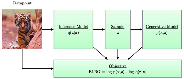
Example 4 提到 VAE 的 forward path 如下圖右：input $x$ 經過 encoder NN $\phi$ 產生 parameters ($\mu, \log \sigma$) of a random variable $\mathbf{z}$ 再 with distribution $q_{\phi}(z\mid x)$. 從 $\mathbf{z}$ 產生 sample f 經過 decoder NN $\theta$ (not shown here). 問題在於 (SGD) back propagation 整條路徑需要是 differentiable. 顯然 random variable $\mathbf{z}$ 的 sample process 不是 differentiable, back propagation 無法 update encoder NN $\phi$.

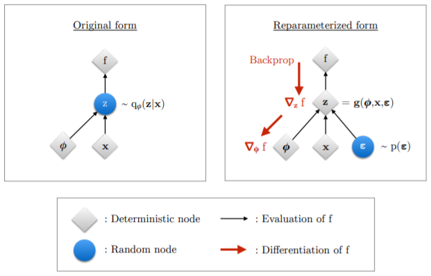
Reparameterization trick 就是為了解決這個問題。How?

1. 把 $\mathbf{z} \sim q_{\phi}(z\mid x)$ 轉換 (differentiable and invertable) 成另一個 random variable $\boldsymbol{\epsilon}$, given $\mathbf{z}$ and $\phi$:

\[\mathbf{z}=\mathbf{g}(\boldsymbol{\epsilon}, \boldsymbol{\phi}, \mathbf{x})\]

where the distribution of random variable $\boldsymbol{\epsilon}$ is indepedent of $\boldsymbol{\phi}, \mathbf{x}$.

1. Gradient of expectation under change of variable

\[\mathbb{E}_{q_{\phi}(\mathbf{z} \mid \mathbf{x})}[f(\mathbf{z})]=\mathbb{E}_{p(\epsilon)}[f(\mathbf{z})]\]

where $\mathbf{z}=\mathbf{g}(\boldsymbol{\epsilon}, \boldsymbol{\phi}, \mathbf{x})$, and the gradient and expectation becomes commutative, 結果如上圖右。

\[\begin{aligned} \nabla_{\phi} \mathbb{E}_{q_{\phi}(\mathbf{z} \mid \mathbf{x})}[f(\mathbf{z})] &=\nabla_{\phi} \mathbb{E}_{p(\boldsymbol{\epsilon})}[f(\mathbf{z})] \\ &=\mathbb{E}_{p(\boldsymbol{\epsilon})}\left[\nabla_{\phi} f(\mathbf{z})\right] \\ & \simeq \nabla_{\phi} f(\mathbf{z}) \end{aligned}\]

更多的數學推導可以參考 ref[Maxwelling], 最後完整的形式如下：

假設 factorized Gaussian encoder

\[\begin{array}{r} q_{\phi}(\mathbf{z} \mid \mathbf{x})=\mathcal{N}\left(\mathbf{z} ; \boldsymbol{\mu}, \operatorname{diag}\left(\boldsymbol{\sigma}^{2}\right)\right): \\ (\boldsymbol{\mu}, \log \boldsymbol{\sigma})=\text { EncoderNeuralNet }_{\boldsymbol{\phi}}(\mathbf{x}) \\ q_{\phi}(\mathbf{z} \mid \mathbf{x})=\prod_{i} q_{\phi}\left(z_{i} \mid \mathbf{x}\right)=\prod_{i} \mathcal{N}\left(z_{i} ; \mu_{i}, \sigma_{i}^{2}\right) \end{array}\]

做完 reparametrization, 我們得到

\[\begin{aligned} \boldsymbol{\epsilon} & \sim \mathcal{N}(0, \mathbf{I}) \\ (\boldsymbol{\mu}, \log \boldsymbol{\sigma}) &=\text { EncoderNeuralNet }_{\phi}(\mathbf{x}) \\ \mathbf{z} &=\boldsymbol{\mu}+\boldsymbol{\sigma} \odot \boldsymbol{\epsilon} \end{aligned}\]

where $\odot$ is the element-wise product. The Jacobian of the transformation from $\boldsymbol{\epsilon}$ to $\mathbf{z}$ is:

\[\log d_{\boldsymbol{\phi}}(\mathbf{x}, \boldsymbol{\epsilon})=\log \left|\operatorname{det}\left(\frac{\partial \mathbf{z}}{\partial \boldsymbol{\epsilon}}\right)\right|=\sum_{i} \log \sigma_{i}\]

and the posterior distribution is:

\[\begin{aligned} \log q_{\phi}(\mathbf{z} \mid \mathbf{x}) &=\log p(\boldsymbol{\epsilon})-\log d_{\phi}(\mathbf{x}, \boldsymbol{\epsilon}) \\ &=\sum_{i} \log \mathcal{N}\left(\epsilon_{i} ; 0,1\right)-\log \sigma_{i} \end{aligned}\]

when $\mathbf{z}=\mathbf{g}(\boldsymbol{\epsilon}, \boldsymbol{\phi}, \mathbf{x})$

Algorithm 1: VAE?

SGD optimization of ELBO. 這裡的 noise 包含 sampling of $p(\boldsymbol{\epsilon})$ 以及 mini-batch sampling.

Data:

$\mathcal{D}$ : Dataset

$q_{\phi}(\mathbf{z}\mid \mathbf{x})$ : Inference model

$p_{\theta}(\mathbf{z}, \mathbf{x})$ : Generative model

Result:

$\theta, \phi$ : Learned parameters

ALG:

($\theta, \phi$) Initialize parameters

while SGD not converged do

$\mathcal{M} \sim \mathcal{D}$ (Random minibatch of data)

$\boldsymbol{\epsilon} \sim p(\boldsymbol{\epsilon})$ (Random noise for every datapoint in $\mathcal{M}$)

Compute $\tilde{\mathcal{L}}_{\theta, \phi}(\mathcal{M}, \boldsymbol{\epsilon})$ and gradients $\nabla_{\boldsymbol{\theta}, \phi} \tilde{\mathcal{L}}_{\boldsymbol{\theta}, \phi}(\mathcal{M}, \boldsymbol{\epsilon})$ ​ Update $\theta$ and $\phi$ using SGD optimizer

end

更複雜的推廣 full-covariance Gaussian encoder $\mathbf{z}=\boldsymbol{\mu}+\mathbf{L} \boldsymbol{\epsilon}$ 可以參考 Appendix B.

Joint distribution of native distribution with hidden variable $z$ [Ref: 科學空間]

VAE 剛才的邏輯是從 marginal likelihood = ELBO + Gap. 接著 focus on maximizing ELBO (假設 maximize ELBO 就會自動 minimize Gap in VAE, how to prove?, not in EM). 因為 ELBO = -1 * (VAE loss) for given $x_i$. Maximimize ELBO = Minimize VAE loss for a given $x_i$.

科學空間 [] 一個不同的做法是直接 minimize distance between joint distribution $(x, z)$, i.e. $q_{D,\phi}(x,z)$ where x is the true data distribution (x–> z via encoder) and joint distribution $(x’, z)$, i.e. $p_{\theta}(x,z)$ where x’ is the marginal distribution (z –> x’) generated by decoder.

數學上就是 minimize the KL divergence of $q_{D,\phi}(x,z) = q_{D}(x) q_{\phi}(z\mid x)$ and $p_{\theta}(x,z) = p(z) p_{\theta}(x\mid z)$, [^1].

[^1]: 科學空間 notation: $\tilde{p}(x,z) = \tilde{p}(x) q(z

x)$​​​​ and $p(x,z) = p(x

z) p(z)$​​​​, where $\tilde{p}(x)$​​​ is the native image distribution.

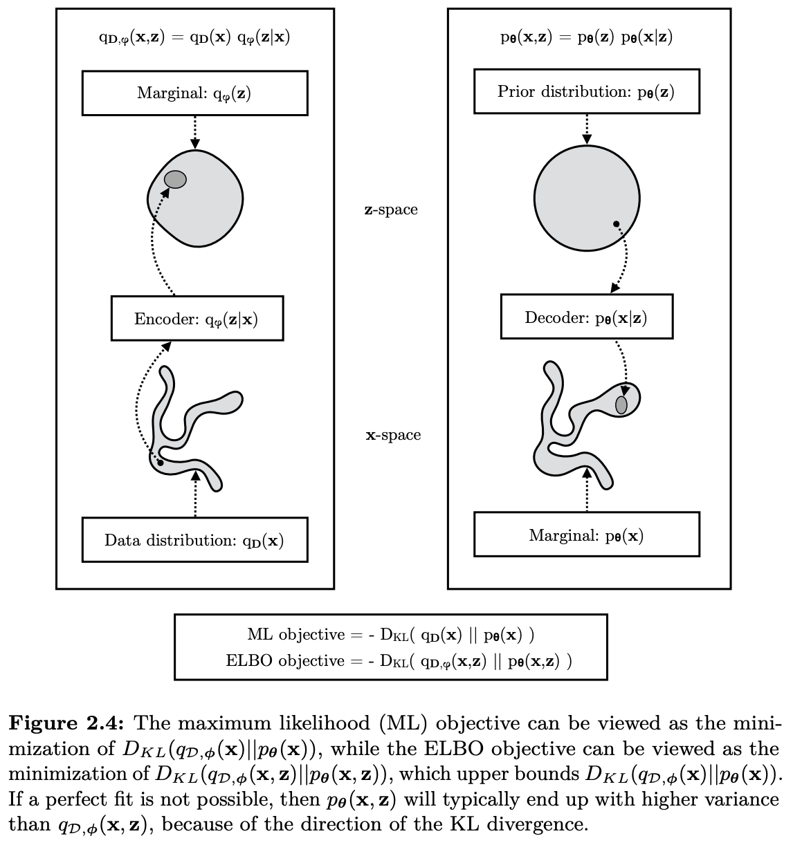
目標就是讓 $p(x, z)$ 儘量逼近 $\tilde{p}(x,z)$, 也就是 minimize 兩個機率分布的距離 (KL divergence).

\[\begin{aligned} D_{K L}(q_{D,\phi}(x, z) \| p_{\theta}(x, z)) &= \iint q_{D,\phi}(x, z) \ln \frac{q_{D,\phi}(x, z)}{p_{\theta}(x, z)} d z d x \\ &=\int q_{D}(x)\left[\int q_{\phi}(z | x) \ln \frac{q_{D}(x) q_{\phi}(z | x)}{p_{\theta}(x, z)} d z\right] d x \\ &=\mathbb{E}_{x \sim q_{D}(x)}\left[\int q_{\phi}(z | x) \ln \frac{q_{D}(x) q_{\phi}(z | x)}{p_{\theta}(x, z)} d z\right] \end{aligned}\]

因為

\[\ln \frac{q_{D}(x) q_{\phi}(z | x)}{p_{\theta}(x, z)}=\ln q_{D}(x)+\ln \frac{q_{\phi}(z | x)}{p_{\theta}(x, z)}\] \[\begin{aligned} \mathbb{E}_{x \sim q_{D}(x)}\left[\int q_{\phi}(z | x) \ln q_{D}(x) d z\right] &=\mathbb{E}_{x \sim q_{D}(x)}\left[\ln q_{D}(x) \int q_{\phi}(z | x) d z\right] \\ &=\mathbb{E}_{x \sim q_{D}(x)}[\ln q_{D}(x)] \\&= -H_X \end{aligned}\]

注意這裡的 $q_{D}(x)$ 是根據樣本 $x_1,x_2,…,x_n$ 確定的關於 $x$ 的分布，儘管我們不一定能準確寫出它的形式，但它是確定的、存在的，因此這一項只是一個常數, actually the entropy of X, $H_X$, not related to z，所以可以寫出 loss function (越小越好，但大於等於 0)：

\[\mathcal{L}=D_{K L}(q_{D,\phi}(x, z) \| p_{\theta}(x, z)) + H_X =\mathbb{E}_{x \sim q_{D}(x)}\left[\int q_{\phi}(z | x) \ln \frac{q_{\phi}(z | x)}{p_{\theta}(x, z)} d z\right] \ge H_X\]

By $p_{\theta}(x,z) = p_{\theta}(x|z) p(z)$ \(\begin{aligned} \mathcal{L} &=\mathbb{E}_{x \sim q_{D}(x)}\left[\int q_{\phi}(z | x) \ln \frac{q_{\phi}(z | x)}{p_{\theta}(x | z) p(z)} d z\right] \\ &=\mathbb{E}_{x \sim q_{D}(x)}\left[-\int q_{\phi}(z | x) \ln p_{\theta}(x | z) d z+\int q_{\phi}(z | x) \ln \frac{q_{\phi}(z | x)}{p(z)} d z\right] \\ &=\mathbb{E}_{x \sim q_{D}(x)} \left[\mathbb{E}_{z \sim q_{\phi}(z | x)}[-\ln p_{\theta}(x | z)]+ D_{K L}(q_{\phi}(z | x) \| \,p(z))\right] \end{aligned}\)

**括號內的不就是VAE的損失函數嘛？只不過我們換了個符號而已。我們就是要想辦法找到適當的 $q_{\phi}(x

z)$ 和 $p(z)$使得 $\mathcal{L}$ 最小化。**

幾個點：

• $D_{K L}(p(x), q(x)) \ge 0$, 等號成立 when $p(x)=q(x)$.
• Only discrete distribution entropy function $H \ge 0$. 如果是 continuous distribution, $H$ 可以小於 0 (見下文).
• 上式的 $L=D_{K L} + H_X \ge H_X$, the minimum is the entropy of X.

VAE Formulation

三種相似的概念：$x’ \sim x$ where $x’$ is the reconstructed image, and $x$ is the native image. (1) ML (maximum marginal likelihood) ; (2) Minimize KL of $(q_{\phi}(x \mid z) | p_{\theta} (x\mid z) $) ; (3) Maximize ELBO. 這三個 objectives 的關係?

1. 直接 Maximum Likelihood (ML) optimize $\theta$ 讓 $q_{D}(x) \sim p_{\theta}(x)$. 但非常困難 and intractable. Minimize $D_{K L}\left(q_{D}(x) | p_{\theta}(x) \right)$ over all $x$

2. Posterior approximation: $q_{\boldsymbol{\phi}}(\mathbf{z} \mid \mathbf{x}) \sim p_{\boldsymbol{\theta}}(\mathbf{z} \mid \mathbf{x})$ given $x_i$

   Minimize $D_{K L}\left(q_{\boldsymbol{\phi}}(\mathbf{z} \mid \mathbf{x}) | p_{\boldsymbol{\theta}}(\mathbf{z} \mid \mathbf{x})\right)$ => 只有讓 marginal likelihood 接近 ELBO. 好像不夠讓 x’ ~ x. (?)

3. Joint distribution approximation: $q_{D,\phi}(x,z) = q_{D}(x) q_{\phi}(z\mid x)\sim p_{\theta}(x,z) = p(z) p_{\theta}(x\mid z)$

   Minimize $D_{K L}\left(q_{D,\phi}(x,z) | p_{\theta}(x,z) \right) \equiv$ Minimize average VAE loss function over all $x$ $\equiv$ Maximize ELBO

• EM: final ML objective (1): first minimize KL objective (E-step, 2); then maximize ELBO objective (M-step, 3); and iteration
• **VAE: maximize ELBO objective (2)! **

Estimation of Marginal Likelihood (Generative)

在 VAE training $(\theta, \phi)$ 之後，下一步是可以 estimate marginal likelihood, $p_{\theta}(\mathbf{x})$, using important sampling technique. The marginal likelihood likelihood of a datapoint is:

\[\log p_{\boldsymbol{\theta}}(\mathbf{x})=\log \mathbb{E}_{q_{\phi}(\mathbf{z} \mid \mathbf{x})}\left[p_{\boldsymbol{\theta}}(\mathbf{x}, \mathbf{z}) / q_{\phi}(\mathbf{z} \mid \mathbf{x})\right]\]

Taking random samples from $q_{\phi}(\mathbf{z} \mid \mathbf{x})$, a Monte Carlo estimator is:

\[\log p_{\boldsymbol{\theta}}(\mathbf{x}) \approx \log \frac{1}{L} \sum_{l=1}^{L} p_{\boldsymbol{\theta}}\left(\mathbf{x}, \mathbf{z}^{(l)}\right) / q_{\phi}\left(\mathbf{z}^{(l)} \mid \mathbf{x}\right)\]

where each $\mathbf{z}^{(l)}\sim q_{\phi}(\mathbf{z} \mid \mathbf{x})$ is a random sample from the inference (i.e. encoder) model.

如果讓 $L$ 足夠大 $L\to\infty$，這個 Monte Carlo approximate estimator 就會越來越接近 marginal likelihood estimation.

相反 $L=1$， 基本就變成 VAE 的 ELBO estimation.

先停在這裡。

Appendix

Appendix A: VAE Loss Function Using Mutual Information

VAE 的 loss function [Wiki] and block diagram \(\begin{align} l_{i}(\theta, \phi)=-E_{z \sim q_{\phi}\left(z | x_{i}\right)}\left[\log p_{\theta}(x_{i} | z)\right]+D_{K L} \left(q_{\phi}(z | x_{i}) \|\,p(z)\right) \end{align}\)

上式第一項是 reconstruction loss, 可以從 Gaussian distribution assumption 清楚看出。第二項的 KL divergence forces encoder 接近 $N(0, I)$, 是一個重要的 regularization term to prevent probabilistic VAE 變成 deterministic Autoencoder.

上式只針對特定 $x_i$, 完整的 loss function 還需要包含 $x_i$ distribution $q_{D}(x)$ 如下。

Total loss function 對於 input distribution $q_{D}(x)$ 積分。 $q_{D}(x)$ 大多不是 normal distribution.

\[\begin{align*} \mathcal{L}&=\mathbb{E}_{x \sim q_{D}(x)}\left[\mathbb{E}_{z \sim q_{\phi}(z | x)}[-\log p_{\theta}(x | z)]+D_{K L}(q_{\phi}(z | x) \| \,p(z))\right] \\ &=\mathbb{E}_{x \sim q_{D}(x)} \mathbb{E}_{z \sim q_{\phi}(z | x)}[-\log p_{\theta}(x | z)]+ \mathbb{E}_{x \sim q_{D}(x)} D_{K L}(q_{\phi}(z | x) \| \,p(z)) \\ &= - \iint q_{D}(x) q_{\phi}(z | x) [\log p_{\theta}(x | z)] dz dx + \mathbb{E}_{x \sim q_{D}(x)} D_{K L}(q_{\phi}(z | x) \| \,p(z)) \end{align*}\]

因為 $\mathbb{E}{x \sim q{D}(x)}\left[\int q_{\phi}(z

x) \ln q_{D}(x) d z\right] = -H_X$

\[\begin{align*} \mathcal{L}&= - \iint q_{D}(x) q_{\phi}(z | x) [\log p_{\theta}(x | z)] dz dx + \mathbb{E}_{x \sim q_{D}(x)} D_{K L}(q_{\phi}(z | x) \| \,p(z)) \\ &= - \iint q_{\phi}(z, x) \log \frac{ p_{\theta}(x, z)}{q_{D}(x) p(z)} dz dx + H_X + \mathbb{E}_{x \sim q_{D}(x)} D_{K L}(q_{\phi}(z | x) \| \,p(z)) \\ \end{align*}\]

對 $x$ distribution 積分的完整 loss function, 第一項就不只是 reconstruction loss, 而有更深刻的物理意義。

記得 VAE 的目標是讓 $q_{D}(x) q_{\phi}(z\mid x) \sim p_\theta(x\mid z) p(z) \to q_{\phi}(z, x) \sim p_\theta(z, x)$.

此時再來 review VAE loss function, 上式第一項可以近似為 $(x, z)$ 的 mutual information! 第二項是 constant. 第三項是 (average) regularization term, always positive (>0), 避免 approximate posterior 變成 deterministic.

Optimization target: maximize mutual information and minimize regularization loss, 這是 trade-off.

\[\begin{align*} \mathcal{L}& \sim - I(z, x) + H_X + \mathbb{E}_{x \sim q_{D}(x)} D_{K L}(q_{\phi}(z | x) \| \,p(z)) \\ \end{align*}\]

Q: 實務上 $z$ 只會有部分的 $x$ information, i.e. $I(x, z) < H(x) \text{ or } H(z)$. $z$ 產生的 $x’$ 也只有部分部分的 $x$ information. $x’$ 真的有可能復刻 $x$ 嗎？
A: 復刻的目標一般是 $x$ and $x’$ distribution 儘量接近，也就是 KL divergence 越小越好。這和 mutual information 是兩件事。例如兩個 independent $N(0, 1)$ normal distributions 的 KL divergence 為 0，但是 mutual information, $I$, 為 0. Maximum mutual information 是 1-1 對應，這不是 VAE 的目的。 VAE 一般是要求 marginal likelihood distribution 或是 posterior distribution 能夠被儘可能近似，而不是 1-1 對應。例如 $x$ 是一張狗的照片，產生 $\mu$ and $\log \sigma$ for $z$, 但是 random sample $z$ 產生的 $x’$ 並不會是狗的照片。

這帶出 machine learning 兩個常見的對抗機制:

1. GAN: 完全分離的 discriminator and generator 的對抗。
2. VAE: encoder/decoder type，注意不是 encoder 和 decoder 的對抗，而是 probabilistic 和 deterministic 的對抗 => maximize mutual information I(z,x) + minimize KL divergence of posterior $p(z\mid x)$ vs. prior $p(z)$ (usually a normal distribution).

(1) 如果 x and z 有一對一 deterministic relationship, I(z, x) = H(z) = H(x) 有最大值。但這會讓 $q_{\phi}(z\mid x)$ 變成 $\delta$ function, 造成 KL divergence 變大。 (2) 如果 x and z 完全 independent, 第二項有最小值，但是 mutual information 最小。最佳值是 trade-off result.

##

Appendix B: Full-covariance Gaussian encoder

\[q_{\phi}(\mathbf{z} \mid \mathbf{x})=\mathcal{N}(\mathbf{z} ; \boldsymbol{\mu}, \boldsymbol{\Sigma})\]

A reparameterization of this distribution is given by:

\[\begin{aligned} &\boldsymbol{\epsilon} \sim \mathcal{N}(0, \mathbf{I}) \\ &\mathbf{z}=\boldsymbol{\mu}+\mathbf{L} \boldsymbol{\epsilon} \end{aligned}\]

where $\mathbf{L}$ is a lower (or upper) triangular matrix, with non-zero entries on the diagonal. The off-diagonal elements defines the correlations of elements in $\mathbf{z}$.

Goal A - Algorithm 2

Computation of unbiased estimate of single datapoint ELBO for example VAE with a full-covariance Gaussian inference model and a factorized Bernoulli generative model. $\mathbf{L}_{mask}$ is a masking matrix with zeros on and above the diagonal, and ones below the diagonal.

Data:

$\mathbf{x}$ : a datapoint, and optionally other conditioning information

$\boldsymbol{\epsilon}$ : a random sample from $p(\boldsymbol{\epsilon}) = \mathcal{N}(0, \mathbf{I})$

$\boldsymbol{\theta}$ : Generative model parameter

$\boldsymbol{\phi}$ : Inference model parameter

$q_{\phi}(\mathbf{z}\mid \mathbf{x})$ : Inference model

$p_{\theta}(\mathbf{z}, \mathbf{x})$ : Generative model

Result:

$\tilde{\mathcal{L}}$ : unbiased estimate of the signle-datapoint ELBO $\mathcal{L}_{\theta,\phi}(\mathbf{x})$

ALG: \(\begin{align*} &\left(\boldsymbol{\mu}, \log \boldsymbol{\sigma}, \mathbf{L}^{\prime}\right) \leftarrow \text { EncoderNeuralNet }_{\phi}(\mathbf{x}) \\ &\mathbf{L} \leftarrow \mathbf{L}_{\text {mask }} \odot \mathbf{L}^{\prime}+\operatorname{diag}(\boldsymbol{\sigma}) \\ &\boldsymbol{\epsilon} \sim \mathcal{N}(0, \mathbf{I}) \\ &\mathbf{z} \leftarrow \mathbf{L} \boldsymbol{\epsilon}+\boldsymbol{\mu} \\ &\tilde{\mathcal{L}}_{\text {logqz }} \leftarrow-\sum_{i}\left(\frac{1}{2}\left(\epsilon_{i}^{2}+\log (2 \pi)+\log \sigma_{i}\right)\right)_{i} & \triangleright=q_{\boldsymbol{\phi}}(\mathbf{z} \mid \mathbf{x})\\ &\tilde{\mathcal{L}}_{\operatorname{logpz}} \leftarrow-\sum_{i}\left(\frac{1}{2}\left(z_{i}^{2}+\log (2 \pi)\right)\right) & \triangleright=p_{\boldsymbol{\theta}}(\mathbf{z})\\ &\mathbf{p} \leftarrow \text { DecoderNeuralNet }_{\theta}(\mathbf{z}) \\ &\tilde{\mathcal{L}}_{\operatorname{logpx}} \leftarrow \sum_{i}\left(x_{i} \log p_{i}+\left(1-x_{i}\right) \log \left(1-p_{i}\right)\right) & \triangleright=p_{\boldsymbol{\theta}}(\mathbf{x} \mid \mathbf{z}) \\ &\tilde{\mathcal{L}}=\tilde{\mathcal{L}}_{\operatorname{logpx}}+\tilde{\mathcal{L}}_{\operatorname{logpz}}-\tilde{\mathcal{L}}_{\operatorname{logqz}} \end{align*}\) 第一項 loss function 就是 reconstruction loss, 不過是 Bernoulli distribution，可以視爲 black-and-white image. 第二項是 prior loss gauge how far it is from normal distribution? 第三項是 regularization term? $\sigma = 1$ 是 minimum loss point.