Math AI - Diffusion Generative Model Extended from VAE

Introduction

最近一段時間，AI 作畫紅的一塌糊塗。

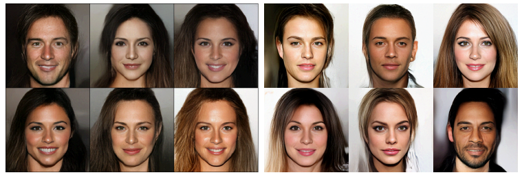
在你驚嘆 AI 繪畫能力的同時，可能還不知道的是，擴散模型在其中起了大作用。就拿熱門模型 OpenAI 的 DALL·E 2 來說，只需輸入簡單的 text prompt，它就可以生成多張 1024*1024 的高清圖象。

在 DALL·E 2 公佈沒多久，谷歌隨後發佈了 Imagen，這是一個 text-to-image 的 AI 模型，它能夠通過給定的 text 描述生成該場景下逼真的圖象。

就在前幾天，Stability.Ai 公開發佈 text-to-image 模型 Stable Diffusion 的最新版本，其生成的圖象達到商用級別。

自 2020 年谷歌發佈 DDPM 以來，擴散模型就逐漸成為生成領域的一個新熱點。之後 OpenAI 推出 GLIDE、ADM-G 模型等，都讓擴散模型火紅。

很多研究者認為，基於擴散模型的文本圖象生成模型不但參數量小，生成的圖象質量卻更高，大有要取代 GAN 的勢頭。

不過，擴散模型背後的數學公式讓許多研究者望而卻步，眾多研究者認為，其比 VAE、GAN 要難理解得多。

近日，來自 Google Research 的研究者撰文《 Understanding Diffusion Models: A Unified Perspective 》，本文以極其詳細的方式展示了擴散模型背後的數學原理，目的是讓其他研究者可以跟隨並瞭解擴散模型是什麼以及它們是如何工作的。最近 generative model 非常紅。特別是 diffusion generative model.

Diffusion generative model 是新的

Summary:

VAE 或是 HVAE 的 objective 是 maximize ELBO.
ELBO 包含三項：reconstruction loss + prior matching loss + denoise matching loss.
第三項 (denoise matching term) 是 VDM optimization 的 objective.
所以 HVAE 和 VDM 相關，或是說 VDM 是 HVAE 的特例。

VAE Recap

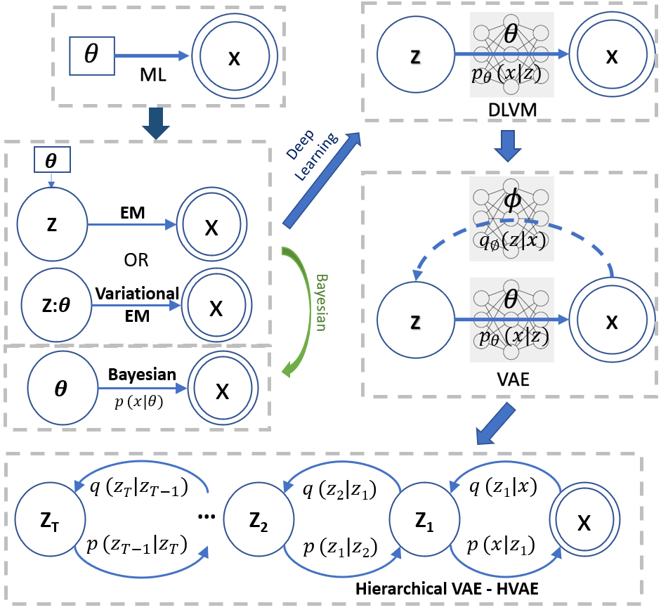
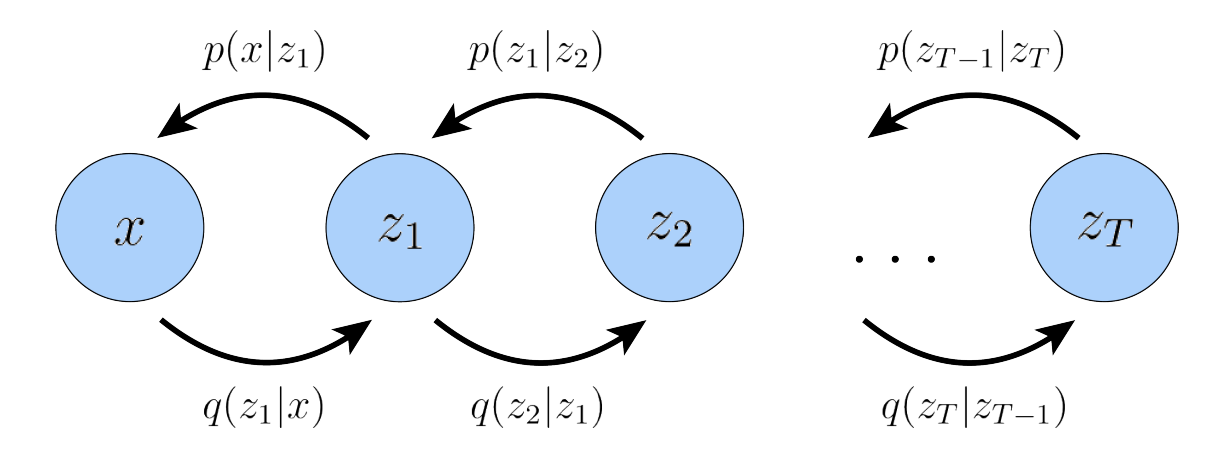
我們從 Bayesian model of two random variable 開始，如下圖。

Forward path 是 likelihood, backward path 是 posterior.

術語 (terminology) 和解讀

先説結論 from Bayesian formula: Posterior $\propto$ Likelihood x Prior $\to p(\theta

\mathbf{x}) \propto {p(\mathbf{x}

\theta)\times p(\theta)}$

一般我們忽略分母的 $p(\mathbf{x})$ ，因為它和要 estimate 的 $\theta$ distribution (or parameter) 無關，視為常數忽略。
很好記: 事後 = 事前 x 喜歡 (likelihood).

Random variable $\mathbf{x}$ : post (事後) observations, (post) evidence. $p(x)$ 稱為 evidence distribution or marginal likelihood, NOT prior distribution.
Random variable $\theta$, or $\mathbf{z}$ : prior (事前, 先驗) 並且是 hidden variable (i.e. not evidence). 擴展我們在 maximum likelihood 的定義，從 parameter 變成 random variable. $p(\theta)$ 稱為 prior distribution.
- 注意 prior 是 distribution, 不會出現在 ML, 因為 $\theta$ 在 ML 是 parameter. 只有在 Bayesian 才有 prior (distribution)!

Conditional distribution $p(\mathbf{x}

\theta)$ : likelihood (或然率)。擴展我們在 maximum likelihood 的定義，從 parameter dependent distribution or function 變成 conditional distribution.

Conditional distribution $p(\theta \mathbf{x})$ ： posterior, 事後機率。就是我們想要求解的東西。
- 注意 posterior 是 conditional distribution. 有人會以為 $p(\theta)$ 是 prior distribution (correct), $p(\mathbf{x})$ 是 posterior distribution (wrong!)
- Posterior 不會出現在 ML, 因為 $\theta$ 在 ML 是 parameter. 只有在 Bayesian 才會討論 posterior (distribution)!
什麽是 Variational? 就是 maximize (or minimize) a family of functions in a integration (or expectation).

算法和觀念演進：From Parameter Estimation (ML) to Generative Model (VAE)

ML (Maximum Likelihood, with a fixed and unknown parameter $\theta$) $\to\,$EM or variational EM : 天才之處在引入 hidden random variable $\mathbf{z}$ with distribution controlled by a parameter $\theta$. 問題是 $p(\mathbf{x},\mathbf{z};\theta)$ 的 joint distribution 到底是什麽? 只有在很簡單的情況下才能得到 $p(\mathbf{x}, \mathbf{z}; \theta)$, 見前文 “MLE to EM “. 大多情況下非常複雜沒有 close form.

(Variational) EM 引入 hidden random variable 已經是半步的 Bayesian. 接下來有兩個發展：

Bayesian (理論派): 直接把 parameter $\theta$ 變成 random variable. 看起來很直觀，常用於理論推導證明 (e.g. ELBO)。但是 $\theta$ 到底是什麽 distribution 並不直觀，也沒有簡單方法得出。

Deep Learning (實做派): 天才之處在固定一個簡單的 $\mathbf{z}$ distribution, 如 N(0, I), 把 $\theta$ 從一個 簡單的 “parameter” 換成一個複雜的 neural network “mapping/decoder”, $p_{\theta}(\mathbf{x}

\mathbf{z})$ 代替原來 EM 無法計算的 $p(\mathbf{x}, \mathbf{z};\theta) = p_{\theta}(\mathbf{x}

\mathbf{z}) p(\mathbf{z})$ distribution. 也就是把複雜的事情交給 neural network $\theta.$ 這稱爲 DLVM (Deep Learning Variable Model).

如何得到這個複雜的 neural network $\theta$ ? 當然是用學習的方法訓練出這個複雜的 neural network decoder $\theta$. 問題是我們只有 $\mathbf{x}$ observations/evidences, 沒有 hidden data $\mathbf{z}$, 如何學習?

DLVM $\to$ VAE : 天才之處在引入另一個 neural network encoder $\phi$ 近似 intractable posterior $q_{\phi}(\mathbf{z}

\mathbf{x}) \approx p(\mathbf{z}

\mathbf{x})$. 再加上 loss function 就可以同時 train encoder and decoder neural network.

VAE Weakness

VAE $\to$ Hierarchical VAE : 從一個 hidden variable 推廣到多個 hidden variables 似乎是自然的想法。但是有什麽好處？

這和 VAE 的不足之處有關。

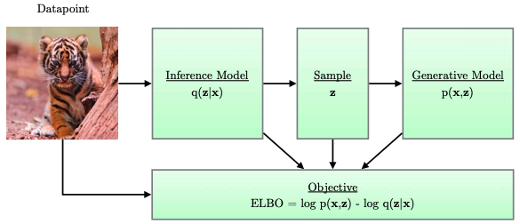
VAE 引入的 hidden variable $\mathbf{z}$, 其直觀 (物理) 意義是 lower dimension feature distribution of $\mathbf{x}$. 重點是如何讓 $\mathbf{z}$ 和 $\mathbf{x}$ 有關係或是讓 $\mathbf{z}$ 學到 $\mathbf{x}$? 一般是要找到 joint pdf $p(\mathbf{x}, \mathbf{z})$ 或是 conditional pdf (i.e. posterior) $q_{\phi}(\mathbf{z}

\mathbf{x}) \approx p(\mathbf{z}

\mathbf{x})$. 問題是這兩個都不容易得到。 VAE 從 variational EM 得到靈感，定義 ELBO (Elbow, Evidence Lower BOund)！

Instead of finding joint pdf or posterior, 定義 \(\begin{align} \log p_{\boldsymbol{\theta}}(\mathbf{x}) &=\mathbb{E}_{q_{\phi}(\mathbf{z} \mid \mathbf{x})}\left[\log p_{\boldsymbol{\theta}}(\mathbf{x})\right] \nonumber\\ &=\mathbb{E}_{q_{\phi}(\mathbf{z} \mid \mathbf{x})}\left[\log \left[\frac{p_{\boldsymbol{\theta}}(\mathbf{x}, \mathbf{z})}{p_{\boldsymbol{\theta}}(\mathbf{z} \mid \mathbf{x})}\right]\right] \nonumber\\ &=\mathbb{E}_{q_{\boldsymbol{\phi}}(\mathbf{z} \mid \mathbf{x})}\left[\log \left[\frac{p_{\boldsymbol{\theta}}(\mathbf{x}, \mathbf{z})}{q_{\boldsymbol{\phi}}(\mathbf{z} \mid \mathbf{x})} \frac{q_{\boldsymbol{\phi}}(\mathbf{z} \mid \mathbf{x})}{p_{\boldsymbol{\theta}}(\mathbf{z} \mid \mathbf{x})}\right]\right] \nonumber\\ &=\underbrace{\mathbb{E}_{q_{\boldsymbol{\phi}}(\mathbf{z} \mid \mathbf{x})}\left[\log \left[\frac{p_{\boldsymbol{\theta}}(\mathbf{x}, \mathbf{z})}{q_{\boldsymbol{\phi}}(\mathbf{z} \mid \mathbf{x})}\right]\right]}_{=\mathcal{L}_{\theta,\phi}{(\boldsymbol{x}})\,\text{, ELBO}}+\underbrace{\mathbb{E}_{q_{\phi}(\mathbf{z} \mid \mathbf{x})}\left[\log \left[\frac{q_{\boldsymbol{\phi}}(\mathbf{z} \mid \mathbf{x})}{p_{\boldsymbol{\theta}}(\mathbf{z} \mid \mathbf{x})}\right]\right]}_{=D_{K L}\left(q_{\boldsymbol{\phi}}(\mathbf{z} \mid \mathbf{x}) \| p_{\boldsymbol{\theta}}(\mathbf{z} \mid \mathbf{x})\right)} \label{eqELBO} \end{align}\) $\eqref{eqELBO}$ 的第一項就是 ELBO. 可以進一步分解如下式 $\eqref{eqLoss}$。(-1) x ELBO 就是 VAE 的 loss function. 第一項對應 reconstruction loss, 第二項對應 encoder posterior distribution 和 $z$ distribution, $N(0, I)$的 gap. \(\begin{align} \mathbb{E}_{q_\phi(\boldsymbol{z} \mid \boldsymbol{x})}\left[\log \frac{p(\boldsymbol{x}, \boldsymbol{z})}{q_\phi(\boldsymbol{z} \mid \boldsymbol{x})}\right] &=\mathbb{E}_{q_\phi(\boldsymbol{z} \mid \boldsymbol{x})}\left[\log \frac{p_{\boldsymbol{\theta}}(\boldsymbol{x} \mid \boldsymbol{z}) p(\boldsymbol{z})}{q_{\boldsymbol{\phi}}(\boldsymbol{z} \mid \boldsymbol{x})}\right] \nonumber\\ &=\mathbb{E}_{q_\phi(\boldsymbol{z} \mid \boldsymbol{x})}\left[\log p_{\boldsymbol{\theta}}(\boldsymbol{x} \mid \boldsymbol{z})\right]+\mathbb{E}_{q_\phi(\boldsymbol{z} \mid \boldsymbol{x})}\left[\log \frac{p(\boldsymbol{z})}{q_{\boldsymbol{\phi}}(\boldsymbol{z} \mid \boldsymbol{x})}\right] \nonumber\\ &=\underbrace{\mathbb{E}_{q_\phi(\boldsymbol{z} \mid \boldsymbol{x})}\left[\log p_{\boldsymbol{\theta}}(\boldsymbol{x} \mid \boldsymbol{z})\right]}_{\text {reconstruction term }}-\underbrace{D_{\mathrm{KL}}\left(q_{\boldsymbol{\phi}}(\boldsymbol{z} \mid \boldsymbol{x}) \| p(\boldsymbol{z})\right)}_{\text {prior matching term }} \label{eqLoss} \end{align}\)

$\eqref{eqELBO}$ 的第二項是 KL divergence of (近似 posterior) 和 (真正 posterior) . 這個 gap 永遠大於 0.

在 VAE training (or learning) 時，藉著 maximize 第一項 ELBO (可以證明等同 minimize VAE loss function), 就可以讓 $\mathbf{z}$ 透過 $\theta, \phi$ (encoder, decoder) 儘量學習到 $\mathbf{x}$ 的 low dimension feature! 如下圖。

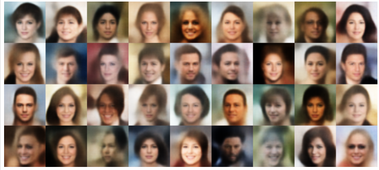
VAE (2014) 理論聽起來完美。不過 VAE 基本沒有用於 generative model (for image or others)，只做爲 baseline for comparison (GAN 是之前 image generation 的主流), 代表 VAE 仍有問題要改善。

EVB generative model 產生的 image 通常比較模糊，如下圖 [@suPowerfulNVAE2020]。可能原因：(a) 上式 KL divergence gap 永遠大於 0 ; (b) feature space, 也就是 $\mathbf{z}$ domain 的不同 features overlapping 所以造成 image 模糊。
一般 generative model 需要支持 Conditional generative model，例如輸入 text 或是 image 產生對應的 image, 而不只是產生 random image. VAE 只有一個 z 似乎不夠？

VAE Next Step : Multiple Hidden Variables

VAE的相關改進：(1) VAE和GAN結合，GAN的缺點是訓練不穩定; (2) VAE和 flow 模型結合 f-VAE; (3) VQ-VAE : vector quantized VAE. (2) 和 (3) 對於 VAE generative model 的改善相對有限。

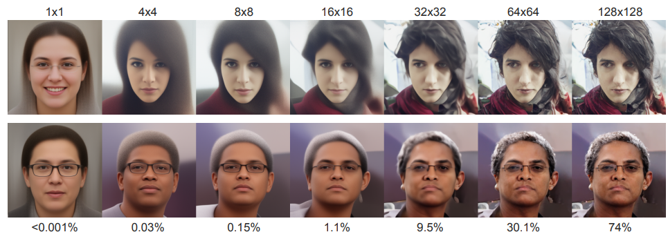
下一個自然的方向就是 multiple hidden variables 通稱為 HVAE - Hierarchical VAE, 例如 NVAE 和 HVAE.

下圖是 [@vahdatNVAEDeep2021] and [@childVeryDeep2021] 的結果，效果很驚艷。細節參考 papers, 沒有假設 Markovian.

HVAE 特例 - Markovian Hidden Variables : Link to Diffusion Model

這裏用一種連結方式如圖一的 Markovian hidden variables 爲例 [@luoUnderstandingDiffusion2022]。

Joint distribution and posterior 可以用 Markov chain rule 如下： $\begin{align} p\left(\boldsymbol{x}, \boldsymbol{z}_{1: T}\right)=p\left(\boldsymbol{z}_T\right) p_{\boldsymbol{\theta}}\left(\boldsymbol{x} \mid \boldsymbol{z}_1\right) \prod_{t=2}^T p_{\boldsymbol{\theta}}\left(\boldsymbol{z}_{t-1} \mid \boldsymbol{z}_t\right) \\ q_{\boldsymbol{\phi}}\left(\boldsymbol{z}_{1: T} \mid \boldsymbol{x}\right)=q_{\boldsymbol{\phi}}\left(\boldsymbol{z}_1 \mid \boldsymbol{x}\right) \prod_{t=2}^T q_{\boldsymbol{\phi}}\left(\boldsymbol{z}_t \mid \boldsymbol{z}_{t-1}\right) \end{align}$

Then, we can easily extend the ELBO to be:

\[\begin{align*} \log p(\boldsymbol{x}) &=\log \int p\left(\boldsymbol{x}, \boldsymbol{z}_{1: T}\right) d \boldsymbol{z}_{1: T} & & \text { (Apply Equation 1) } \\ &=\log \int \frac{p\left(\boldsymbol{x}, \boldsymbol{z}_{1: T}\right) q_{\boldsymbol{\phi}}\left(\boldsymbol{z}_{1: T} \mid \boldsymbol{x}\right)}{q_\phi\left(\boldsymbol{z}_{1: T} \mid \boldsymbol{x}\right)} d \boldsymbol{z}_{1: T} & &\text { (Multiply by } \left.1=\frac{q_{\boldsymbol{\phi}}\left(\boldsymbol{z}_{1: T} \mid \boldsymbol{x}\right)}{q_{\boldsymbol{\phi}}\left(\boldsymbol{z}_{1: T} \mid \boldsymbol{x}\right)}\right) \\ &=\log \mathbb{E}_{q_\phi\left(\boldsymbol{z}_{1: T} \mid \boldsymbol{x}\right)}\left[\frac{p\left(\boldsymbol{x}, \boldsymbol{z}_{1: T}\right)}{q_{\boldsymbol{\phi}}\left(\boldsymbol{z}_{1: T} \mid \boldsymbol{x}\right)}\right] & & \text { (Definition of Expectation) } \\ & \geq \mathbb{E}_{q_\phi\left(\boldsymbol{z}_{1: T} \mid \boldsymbol{x}\right)}\left[\log \frac{p\left(\boldsymbol{x}, \boldsymbol{z}_{1: T}\right)}{q_{\boldsymbol{\phi}}\left(\boldsymbol{z}_{1: T} \mid \boldsymbol{x}\right)}\right] & & \text { (Apply Jensen's Inequality) } \end{align*}\]

We can then plug our joint distribution and posterior into above ELBO to produce an alternate form:

\[\begin{align} \mathbb{E}_{q_\phi\left(\boldsymbol{z}_{1: T} \mid \boldsymbol{x}\right)}\left[\log \frac{p\left(\boldsymbol{x}, \boldsymbol{z}_{1: T}\right)}{q_{\boldsymbol{\phi}}\left(\boldsymbol{z}_{1: T} \mid \boldsymbol{x}\right)}\right]=\mathbb{E}_{q_{\boldsymbol{\phi}}\left(\boldsymbol{z}_{1: T} \mid \boldsymbol{x}\right)}\left[\log \frac{p\left(\boldsymbol{z}_T\right) p_{\boldsymbol{\theta}}\left(\boldsymbol{x} \mid \boldsymbol{z}_1\right) \prod_{t=2}^T p_{\boldsymbol{\theta}}\left(\boldsymbol{z}_{t-1} \mid \boldsymbol{z}_t\right)}{q_{\boldsymbol{\phi}}\left(\boldsymbol{z}_1 \mid \boldsymbol{x}\right) \prod_{t=2}^T q_{\boldsymbol{\phi}}\left(\boldsymbol{z}_t \mid \boldsymbol{z}_{t-1}\right)}\right] \label{eqELBO3} \end{align}\]

Variational Diffusion Models (VDM)

VDM 可以視爲 Markovian Hierarchical VAE 具有幾個關鍵：

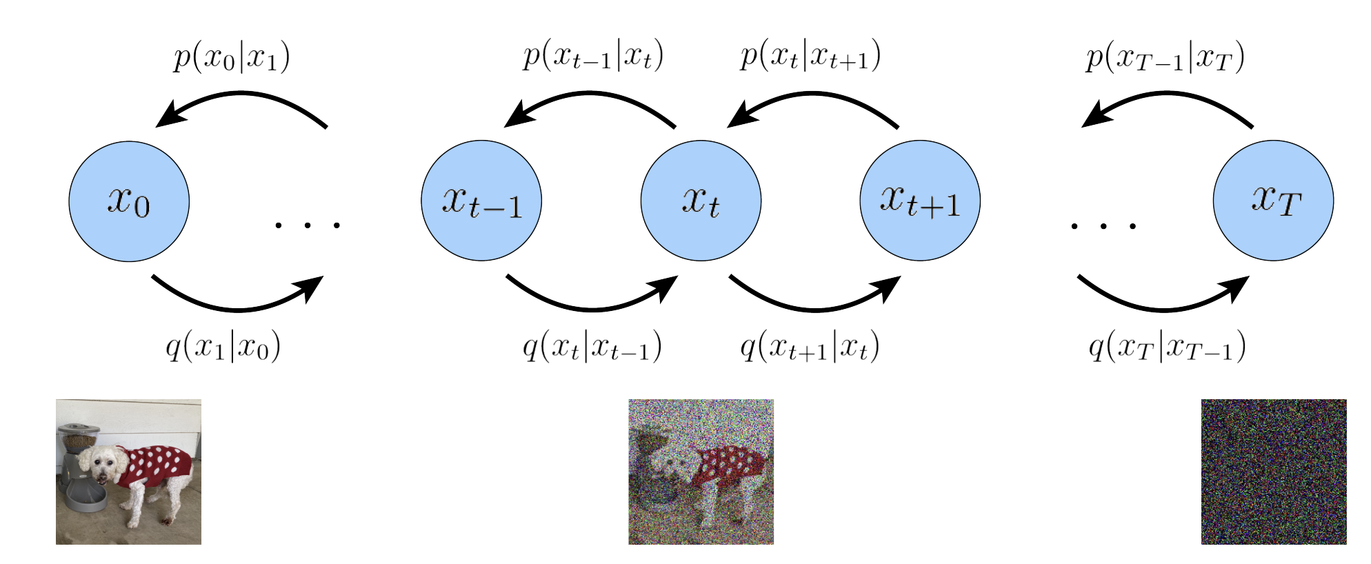
Latent dimension is exactly equal to data dimension, i.e. $\mathbf{z}, \mathbf{x}$ 具有一樣的 dimensions! 所以下圖就全部使用 $\mathbf{x}$ 而不用 $\mathbf{z}$. 這和一般 VAE不同： $\mathbf{z}$ dimension (feature space dimension) 遠小於 $\mathbf{x}$ dimension (observation/evidence dimension).

VDM 的 hidden states 對應 time-step Markovian evolution $\eqref{Markov}$, 而非 NVAE or HVAE 同時存在的 spatial or graphic states.
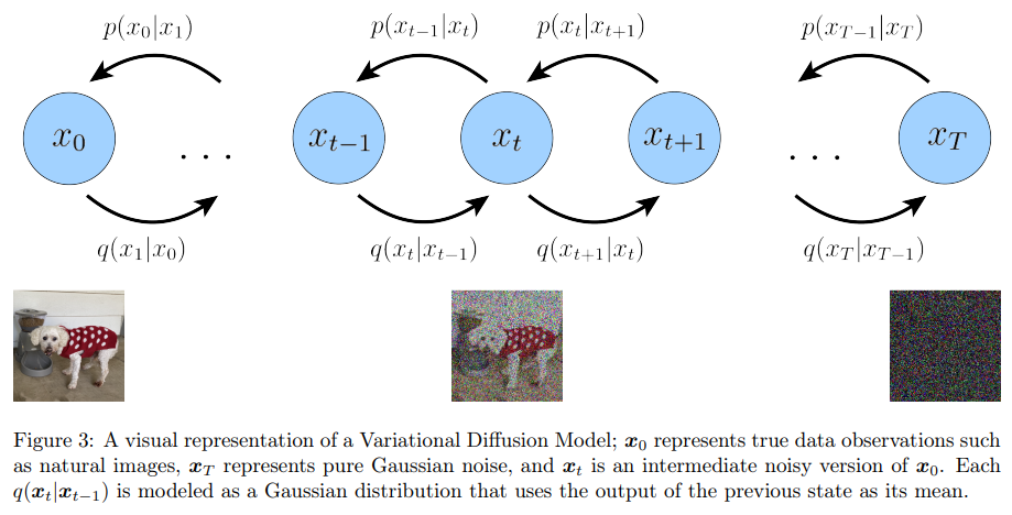
The structure of latent encoder from observation to “noise”, (i.e. $q$ or backward or posterior direction) 已經 pre-defined as linear Gaussian mode. 注意這是 predefined, 不是學習得到的! 換句話說，它是以 previous time-step 輸出為中心的高斯分佈, i.e. 所有的 $q_{\boldsymbol{\phi}}\left(\boldsymbol{x}t \mid \boldsymbol{x}{t-1}\right)$ 都是 linear normal distribution $\eqref{LinGauss}$.

\[\begin{align} q\left(\boldsymbol{x}_{1: T} \mid \boldsymbol{x}_0\right)=\prod_{t=1}^T q\left(\boldsymbol{x}_t \mid \boldsymbol{x}_{t-1}\right) \label{Markov} \end{align}\] \[\begin{align} q\left(\boldsymbol{x}_t \mid \boldsymbol{x}_{t-1}\right)=\mathcal{N}\left(\boldsymbol{x}_t ; \sqrt{\alpha_t} \boldsymbol{x}_{t-1},\left(1-\alpha_t\right) \mathbf{I}\right) \label{LinGauss} \end{align}\]

也就是 normal distribution with mean $\boldsymbol{\mu}t\left(\boldsymbol{x}_t\right)=\sqrt{\alpha_t} \boldsymbol{x}{t-1}$, and variance $\boldsymbol{\Sigma}_t\left(\boldsymbol{x}_t\right)=\left(1-\alpha_t\right) \mathbf{I}$

Why the mean and variance? The form of the coefficients are chosen such that the variance of the latent variables stay at a similar scale; in other words, the encoding process is variance-preserving [@kingmaVariationalDiffusion2022].

Latent encoder 最後 time-step T 對應標準高斯分佈 N(0, I), i.e.

\[\begin{align} p\left(\boldsymbol{x}_T\right) = \mathcal{N}(\boldsymbol{x}_T ;0, I) \label{eqXt} \end{align}\]

以及 VDM 的 joint distribution

\[\begin{align} p\left(\boldsymbol{x}_{0: T}\right)=p\left(\boldsymbol{x}_T\right) \prod_{t=1}^T p_{\boldsymbol{\theta}}\left(\boldsymbol{x}_{t-1} \mid \boldsymbol{x}_t\right) \end{align}\]

我們同樣可以分解 VDM 的 ELBO from $\eqref{eqELBO3}$ with $\boldsymbol{x}\to \boldsymbol{x}_0, \boldsymbol{z}\to \boldsymbol{x}$ ，得到下式 $\eqref{ELBO2a}.$¹

第一項是 reconstruction loss of $x_0, x_1$ 用於 training，基本和 Vanilla VAE ($T=1$) 類似。

第二項是 posterior $q(x_T

x_{T-1})$ 和 $x_T$ distribution gap. 我們如果讓 $T$ 足夠大，可以讓 $\alpha_{T}\sim 0$, 並讓此項消失。

\[\begin{align} \text{ELBO} &= \mathbb{E}_{q\left(\boldsymbol{x}_{1: T} \mid \boldsymbol{x}_0\right)}\left[\log \frac{p\left(\boldsymbol{x}_{0: T}\right)}{q\left(\boldsymbol{x}_{1: T} \mid \boldsymbol{x}_0\right)}\right] \nonumber \\ &=\underbrace{\mathbb{E}_{q\left(\boldsymbol{x}_1 \mid \boldsymbol{x}_0\right)}\left[\log p_\theta\left(\boldsymbol{x}_0 \mid \boldsymbol{x}_1\right)\right]}_{\text {reconstruction term }}-\underbrace{\mathbb{E}_{q\left(\boldsymbol{x}_{T-1} \mid \boldsymbol{x}_0\right)}\left[D_{\mathrm{KL}}\left(q\left(\boldsymbol{x}_T \mid \boldsymbol{x}_{T-1}\right) \| p\left(\boldsymbol{x}_T\right)\right)\right]}_{\text {prior matching term }} \nonumber \\ &-\sum_{t=1}^{T-1} \underbrace{\mathbb{E}_{q\left(\boldsymbol{x}_{t-1}, \boldsymbol{x}_{t+1} \mid \boldsymbol{x}_0\right)}\left[D_{\mathrm{KL}}\left(q\left(\boldsymbol{x}_t \mid \boldsymbol{x}_{t-1}\right) \| p_\theta\left(\boldsymbol{x}_t \mid \boldsymbol{x}_{t+1}\right)\right)\right]}_{\text {consistency term }} \label{ELBO2a} \end{align}\]

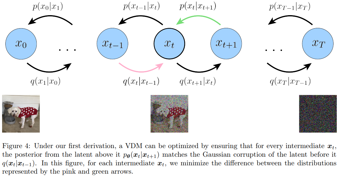
第三項是關鍵項，稱爲 consistency term, VDM 的 cost function 主要被這項 dominant! 可以由下圖的紅綫和綠綫代表，就是要 minimize the gap between forward likelihood and backward posterior at $x_t,t \in [1,T-1]$. 物理的意義就是 image denoise (p-path) 和 image noising (q-path) 要 match. 我們已經 pre-define q-path 是 Gaussian. 也就是要讓 p-path 也近似 Gaussian denoising, equation (7).

第三項的問題是 expectation conditional on two random variables ${x_{t-1}, x_{t+1}}$ 會比較大。因此可以變形一下，expectation condiation on one random variable ${x_0}$ 讓 variance 比較小，如下式 $\eqref{ELBO2}$。 $\begin{align} \text{ELBO} &= \mathbb{E}_{q\left(\boldsymbol{x}_{1: T} \mid \boldsymbol{x}_0\right)}\left[\log \frac{p\left(\boldsymbol{x}_{0: T}\right)}{q\left(\boldsymbol{x}_{1: T} \mid \boldsymbol{x}_0\right)}\right] \nonumber\\ &=\underbrace{\mathbb{E}_{q\left(\boldsymbol{x}_1 \mid \boldsymbol{x}_0\right)}\left[\log p_{\boldsymbol{\theta}}\left(\boldsymbol{x}_0 \mid \boldsymbol{x}_1\right)\right]}_{\text {reconstruction term }}-\underbrace{D_{\mathrm{KL}}\left(q\left(\boldsymbol{x}_T \mid \boldsymbol{x}_0\right) \| p\left(\boldsymbol{x}_T\right)\right)}_{\text {prior matching term }} \nonumber \\ &-\sum_{t=2}^T \underbrace{\mathbb{E}_{q\left(\boldsymbol{x}_t \mid \boldsymbol{x}_0\right)}\left[D_{\mathrm{KL}}\left(q\left(\boldsymbol{x}_{t-1} \mid \boldsymbol{x}_t, \boldsymbol{x}_0\right) \| p_{\boldsymbol{\theta}}\left(\boldsymbol{x}_{t-1} \mid \boldsymbol{x}_t\right)\right)\right]}_{\text {denoising matching term }} \label{ELBO2} \end{align}$

第一項 reconstruction term 和 vanilla VAE (T=1) ELBO 的 reconstruction term 一樣，可以用 Monte Carlo 估計近似 (用 VAE 的方式 training?)。
第二項同樣會趨近 0.
第三項 expectation 只對一個 random variable 所以會比 $\eqref{ELBO2a}$ 小，稱為 denoising match term.

$\eqref{ELBO2}$ 的第三項 DL divergence 的兩邊都是 denoise: p-path 是 denoise $x_t$ to $x_{t-1}$，q-path 也變成 denoise $x_t$ to $x_{t-1}$ but given $x_0$ . 因此第三項稱爲 denoising matching term. 就是考驗 $p$ 和 q denoise 能力是否類似。

這部分參考 https://zhuanlan.zhihu.com/p/565901160

From Probability to Sample

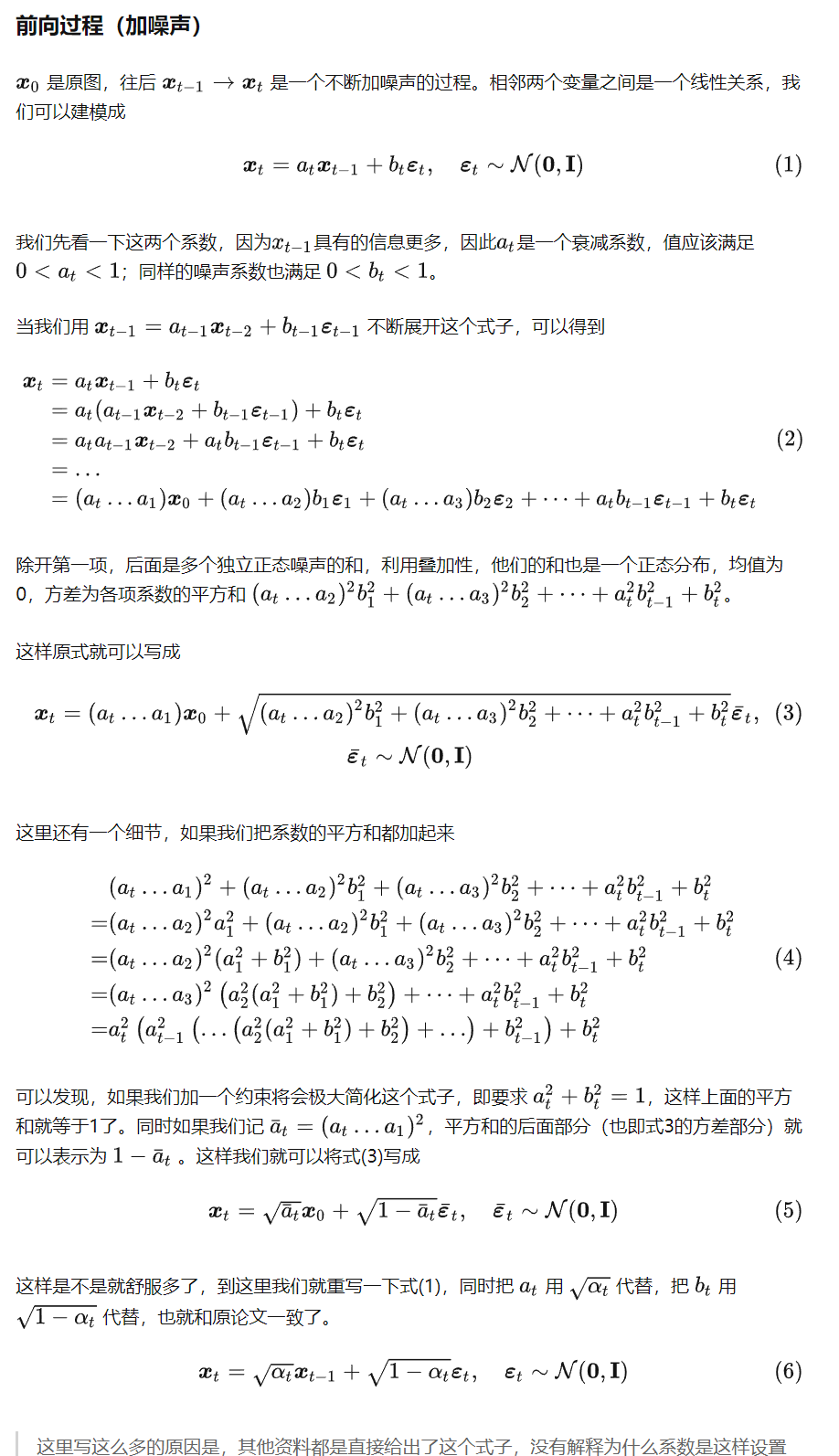
前面都是 probability 理論推導，實際作戰還是用隨機取樣 (Monte Carlo sample) 模擬近似。舉例來說 posterior $\eqref{LinGauss}$ 是 conditional probability : $q\left(\boldsymbol{x}t \mid \boldsymbol{x}{t-1}\right) \sim \mathcal{N}\left(\boldsymbol{x}t ; \sqrt{\alpha_t} \boldsymbol{x}{t-1},\left(1-\alpha_t\right) \mathbf{I}\right)$, 可以用以下 state-space equation 表示，也作為之後用 Monte Carlo sample 的方法。 (Linear Gaussian 看起來像 Kalman filter form)

\[\boldsymbol{x}_t=\sqrt{\alpha_t} \boldsymbol{x}_{t-1}+\sqrt{1-\alpha_t} \boldsymbol{\epsilon} \quad\text{with } \boldsymbol{\epsilon} \sim \mathcal{N}\left(\boldsymbol{\epsilon} ; 0,\mathbf{I}\right)\]

可以看出 given $\boldsymbol{x}{t-1}$, $\boldsymbol{x}_t$ 的 distribution 就是 $\mathcal{N}\left(\sqrt{\alpha_t} \boldsymbol{x}{t-1},\left(1-\alpha_t\right) \mathbf{I}\right)$。注意這裡並沒有假設 $\boldsymbol{x}_t$ 是 Gaussian, 只有假設 $\boldsymbol{\epsilon}$ 是 Gaussian. 可以持續 iteration 如下：

\[\begin{align} \boldsymbol{x}_t&=\sqrt{\alpha_t} \boldsymbol{x}_{t-1}+\sqrt{1-\alpha_t} \boldsymbol{\epsilon}_{t-1}^* \nonumber\\ &=\sqrt{\alpha_t}\left(\sqrt{\alpha_{t-1}} \boldsymbol{x}_{t-2}+\sqrt{1-\alpha_{t-1}} \epsilon_{t-2}^*\right)+\sqrt{1-\alpha_t} \epsilon_{t-1}^* \nonumber\\ &=\sqrt{\alpha_t \alpha_{t-1}} \boldsymbol{x}_{t-2}+\sqrt{\alpha_t-\alpha_t \alpha_{t-1}} \boldsymbol{\epsilon}_{t-2}^*+\sqrt{1-\alpha_t} \epsilon_{t-1}^* \label{Rec}\\ &=\sqrt{\alpha_t \alpha_{t-1}} \boldsymbol{x}_{t-2}+\sqrt{\alpha_t-\alpha_t \alpha_{t-1}+1-\alpha_t} \boldsymbol{\epsilon}_{t-2} \nonumber\\ &=\sqrt{\alpha_t \alpha_{t-1}} \boldsymbol{x}_{t-2}+\sqrt{1-\alpha_t \alpha_{t-1}} \boldsymbol{\epsilon}_{t-2} \nonumber\\ &=\ldots \nonumber\\ &=\sqrt{\prod_{i=1}^t \alpha_i} \boldsymbol{x}_0 +\sqrt{1-\prod_{i=1}^t \alpha_i }\boldsymbol{\epsilon}_0 \nonumber\\ &=\sqrt{\bar{\alpha}_t} \boldsymbol{x}_0+\sqrt{1-\bar{\alpha}_t} \boldsymbol{\epsilon}_0 \label{xt} \end{align}\]

也就是如下的 conditional distribution.

\[\begin{align} q\left(\boldsymbol{x}_t \mid \boldsymbol{x}_{0}\right) &\sim \mathcal{N}\left(\boldsymbol{x}_t ; \sqrt{\bar{\alpha}_t} \boldsymbol{x}_0,\left(1-\bar{\alpha}_t\right) \mathbf{I}\right) \label{xtGauss} \end{align}\]

注意 conditional distribution 是 Gaussian 並不代表 $\boldsymbol{x}_t$ 是 Gaussian. 顯然 $\boldsymbol{x}_0$ (image distribution) 一定不是 Gaussian. 但是 $\boldsymbol{x}_T$ (假設) 是標準高斯分佈 N(0,I) in $\eqref{eqXt}$. 如何解釋從 Non-Gaussian (t=0) 轉變成 Gaussian (t=T) 這個矛盾？

這可以用通訊類比！原始的信號 (t=0) 如聲音分佈是 Non-Gaussian distribution. 當 t 變大對應增加 additive Gaussian noise, SNR (signal-to-noise ratio) 開始變小，聲音加 noise 信號的分佈還是 Non-Gaussian。但 noise 越來越大，SNR 越來越小，最後 (t=T) 的分佈基本就是 Gaussian noise.

回到 $\eqref{ELBO2}$ 的第三項 denoising matching term: 因為 q-path 的 conditional distribution 是 Gaussian process, 可以進一步解出 close form 如下 (Appendix B)，當然也是 Gaussian distribution.

\[\begin{align} &q\left(\boldsymbol{x}_{t-1} \mid \boldsymbol{x}_t, \boldsymbol{x}_0\right)=\frac{q\left(\boldsymbol{x}_t \mid \boldsymbol{x}_{t-1}, \boldsymbol{x}_0\right) q\left(\boldsymbol{x}_{t-1} \mid \boldsymbol{x}_0\right)}{q\left(\boldsymbol{x}_t \mid \boldsymbol{x}_0\right)} \nonumber\\ &=\frac{\mathcal{N}\left(\boldsymbol{x}_t ; \sqrt{\alpha_t} \boldsymbol{x}_{t-1},\left(1-\alpha_t\right) \mathbf{I}\right) \mathcal{N}\left(\boldsymbol{x}_{t-1} ; \sqrt{\bar{\alpha}_{t-1}} \boldsymbol{x}_0,\left(1-\bar{\alpha}_{t-1}\right) \mathbf{I}\right)}{\mathcal{N}\left(\boldsymbol{x}_t ; \sqrt{\bar{\alpha}_t} \boldsymbol{x}_0,\left(1-\bar{\alpha}_t\right) \mathbf{I}\right)}\nonumber \\ &\propto \mathcal{N}(\boldsymbol{x}_{t-1} ; \underbrace{\frac{\sqrt{\alpha_t}\left(1-\bar{\alpha}_{t-1}\right) \boldsymbol{x}_t+\sqrt{\bar{\alpha}_{t-1}}\left(1-\alpha_t\right) \boldsymbol{x}_0}{1-\bar{\alpha}_t}}_{\mu_q\left(\boldsymbol{x}_t, \boldsymbol{x}_0\right)}, \underbrace{\left.\frac{\left(1-\alpha_t\right)\left(1-\bar{\alpha}_{t-1}\right)}{1-\bar{\alpha}_t} \mathbf{I}\right)}_{\boldsymbol{\Sigma}_q(t)} \end{align}\]

為了要 minimize the denoise matching term, *我們假設 *p-path 的 conditional probability $p_{\theta}(x_{t-1}

x_t)$ 也是 Gaussian 而且 variance 和 p-path 一樣！**

利用 DL divergence of two Gaussian distribution formula 可以得到下式。問題就簡化成如何讓兩個 Gaussian distribution 的 mean 一樣。神奇的就把 probabilistic 問題變成 deterministic 問題，就是讓

\[\begin{align} & \underset{\boldsymbol{\theta}}{\arg \min } D_{\mathrm{KL}}\left(q\left(\boldsymbol{x}_{t-1} \mid \boldsymbol{x}_t, \boldsymbol{x}_0\right) \| p_{\boldsymbol{\theta}}\left(\boldsymbol{x}_{t-1} \mid \boldsymbol{x}_t\right)\right) \nonumber\\ =& \underset{\boldsymbol{\theta}}{\arg \min } D_{\mathrm{KL}}\left(\mathcal{N}\left(\boldsymbol{x}_{t-1} ; \boldsymbol{\mu}_q, \boldsymbol{\Sigma}_q(t)\right) \| \mathcal{N}\left(\boldsymbol{x}_{t-1} ; \boldsymbol{\mu}_{\boldsymbol{\theta}}, \boldsymbol{\Sigma}_q(t)\right)\right) \nonumber\\ =&\underset{\boldsymbol{\theta}}{\arg \min } \frac{1}{2}\left[\log \frac{\left|\boldsymbol{\Sigma}_q(t)\right|}{\left|\boldsymbol{\Sigma}_q(t)\right|}-d+\operatorname{tr}\left(\boldsymbol{\Sigma}_q(t)^{-1} \boldsymbol{\Sigma}_q(t)\right)+\left(\boldsymbol{\mu}_{\boldsymbol{\theta}}-\boldsymbol{\mu}_q\right)^T \boldsymbol{\Sigma}_q(t)^{-1}\left(\boldsymbol{\mu}_{\boldsymbol{\theta}}-\boldsymbol{\mu}_q\right)\right] \nonumber\\ =& \underset{\boldsymbol{\theta}}{\arg \min } \frac{1}{2}\left[\log 1-d+d+\left(\boldsymbol{\mu}_{\boldsymbol{\theta}}-\boldsymbol{\mu}_q\right)^T \boldsymbol{\Sigma}_q(t)^{-1}\left(\boldsymbol{\mu}_{\boldsymbol{\theta}}-\boldsymbol{\mu}_q\right)\right] \nonumber\\ =& \underset{\boldsymbol{\theta}}{\arg \min } \frac{1}{2 \sigma_q^2(t)}\left[\left\|\boldsymbol{\mu}_{\boldsymbol{\theta}}-\boldsymbol{\mu}_q\right\|_2^2\right] \label{KLDiv} \end{align}\]

where

\[\boldsymbol{\mu}_q\left(\boldsymbol{x}_t, \boldsymbol{x}_0\right)=\frac{\sqrt{\alpha_t}\left(1-\bar{\alpha}_{t-1}\right) \boldsymbol{x}_t+\sqrt{\bar{\alpha}_{t-1}}\left(1-\alpha_t\right) \boldsymbol{x}_0}{1-\bar{\alpha}_t} \label{MeanQ}\]

稱爲 denoising transition mean. And variance $\boldsymbol{\Sigma}_q(t)=\sigma_q^2(t) \mathbf{I}$ with $\sigma_q^2(t)=\frac{\left(1-\alpha_t\right)\left(1-\bar{\alpha}_{t-1}\right)}{1-\bar{\alpha}_t} \label{Sigma}$

As $\boldsymbol{\mu}_{\boldsymbol{\theta}}\left(\boldsymbol{x}_t, t\right)$ also conditions on $\boldsymbol{x}_t$, but not conditions on $\boldsymbol{x}_0$. We can match $\boldsymbol{\mu}_q\left(\boldsymbol{x}_t, \boldsymbol{x}_0\right)$ closely by setting it to the following form:

\[\boldsymbol{\mu}_{\boldsymbol{\theta}}\left(\boldsymbol{x}_t, t\right)=\frac{\sqrt{\alpha_t}\left(1-\bar{\alpha}_{t-1}\right) \boldsymbol{x}_t+\sqrt{\bar{\alpha}_{t-1}}\left(1-\alpha_t\right) \hat{\boldsymbol{x}}_{\boldsymbol{\theta}}\left(\boldsymbol{x}_t, t\right)}{1-\bar{\alpha}_t}\]

where $\hat{\boldsymbol{x}}_{\boldsymbol{\theta}}\left(\boldsymbol{x}_t, t\right)$ is parameterized by a neural network that seeks to predict $\boldsymbol{x}_0$ from noisy image $\boldsymbol{x}_t$ and time index $t$. Then, the optimization problem simplifies to:

因此，優化 VDM 可以歸結為 training a neural network $\theta$ 在加入任意 (Gaussian) noise 可以學習出原來 ground truth image.

如何表示加入任意 noise？可以通過最小化所有 timesteps expectation of KL divergence 近似原來的 ELBO cost function:

\[\underset{\boldsymbol{\theta}}{\arg \min } \mathbb{E}_{t \sim U\{2, T\}}\left[\mathbb{E}_{q\left(\boldsymbol{x}_t \mid \boldsymbol{x}_0\right)}\left[D_{\mathrm{KL}}\left(q\left(\boldsymbol{x}_{t-1} \mid \boldsymbol{x}_t, \boldsymbol{x}_0\right) \| p_{\boldsymbol{\theta}}\left(\boldsymbol{x}_{t-1} \mid \boldsymbol{x}_t\right)\right)\right]\right]\]

Summary:

VAE 或是 HVAE 的 objective 是 maximize ELBO.
ELBO 包含三項：reconstruction loss + prior matching loss + denoise matching loss.
第三項 (denoise matching term) 是 VDM optimization 的 objective.
所以 HVAE 和 VDM 其實相關。或是 VDM 是 HVAE 的特例。

Learning Diffusion Noise Parameter

$\eqref{Denoise}$ 歸結優化 VDM 為 training a neural network $\theta$ 在加入任意 (Gaussian) noise 可以學習出原來 ground truth image，不過還少了前面 scaling factor 的部分。Scaling factor 可以簡化成 SNR 的學習 (?)。

結合 $\eqref{Sigma}$ 和 $\eqref{Denoise}$，可以得到 $\begin{align} &\frac{1}{2 \sigma_q^2(t)} \frac{\bar{\alpha}_{t-1}\left(1-\alpha_t\right)^2}{\left(1-\bar{\alpha}_t\right)^2}\left[\left\|\hat{\boldsymbol{x}}_{\boldsymbol{\theta}}\left(\boldsymbol{x}_t, t\right)-\boldsymbol{x}_0\right\|_2^2\right]\nonumber\\ =&\frac{1}{2 \frac{\left(1-\alpha_t\right)\left(1-\bar{\alpha}_{t-1}\right)}{1-\bar{\alpha}_t}} \frac{\bar{\alpha}_{t-1}\left(1-\alpha_t\right)^2}{\left(1-\bar{\alpha}_t\right)^2}\left[\left\|\hat{\boldsymbol{x}}_{\boldsymbol{\theta}}\left(\boldsymbol{x}_t, t\right)-\boldsymbol{x}_0\right\|_2^2\right]\nonumber\\ =&\frac{1}{2}\left(\frac{\bar{\alpha}_{t-1}}{1-\bar{\alpha}_{t-1}}-\frac{\bar{\alpha}_t}{1-\bar{\alpha}_t}\right)\left[\left\|\hat{x}_{\boldsymbol{\theta}}\left(\boldsymbol{x}_t, t\right)-\boldsymbol{x}_0\right\|_2^2\right] \label{Denoise2} \end{align}$

我們用 SNR(t) 取代 $\bar{\alpha}_t$ 因爲更有物理意義。代入 $\mathrm{SNR} = \frac{\mu^2}{\sigma^2}$ and use $\eqref{xtGauss}$ 得到

\[\mathrm{SNR(t)} = \frac{\bar{\alpha}_t}{1-\bar{\alpha}_t}\]

注意這裏 ignore $x_0$ 的 mean 因爲只是一個 constant scaling constant factor for all $x_t$.

$\eqref{Denoise2}$ 可以改寫如下式：

\[\begin{align} \frac{1}{2 \sigma_q^2(t)} \frac{\bar{\alpha}_{t-1}\left(1-\alpha_t\right)^2}{\left(1-\bar{\alpha}_t\right)^2}\left[\left\|\hat{\boldsymbol{x}}_{\boldsymbol{\theta}}\left(\boldsymbol{x}_t, t\right)-\boldsymbol{x}_0\right\|_2^2\right] \nonumber\\ =\frac{1}{2}(\mathrm{SNR}(t-1)-\mathrm{SNR}(t))\left[\left\|\hat{\boldsymbol{x}}_{\boldsymbol{\theta}}\left(\boldsymbol{x}_t, t\right)-\boldsymbol{x}_0\right\|_2^2\right] \label{SNR} \end{align}\]

一般會把 SNR 再轉換成 exponential form (better to learn or converge?)

\[\mathrm{SNR(t)} = \frac{\bar{\alpha}_t}{1-\bar{\alpha}_t}=\exp \left(-\omega_{\boldsymbol{\eta}}(t)\right)\\ \omega_{\boldsymbol{\eta}}(t) = - \log \mathrm{SNR(t)}\\ \therefore \bar{\alpha}_t=\operatorname{sigmoid}\left(-\omega_\eta(t)\right)\\ \therefore 1-\bar{\alpha}_t=\operatorname{sigmoid}\left(\omega_{\boldsymbol{\eta}}(t)\right)\]

where $\omega_{\boldsymbol{\eta}}(t)$ is modeled as a monotonically increasing neural network with parameters $\boldsymbol{\eta}$.

Question: 所以需要兩個 neural networks? (1) $\theta$ is to learn the denoise with arbitrary noise; (2) $\eta$ is to learn the $\omega_{\eta}(t)$?

三條大路通羅馬

第一條路：優化 VDM 可以歸結為 training a neural network $\theta$ 在加入任意 (Gaussian) noise 可以學習出原來 ground truth image.

第二條路：另一個角度是否可以從 original image ($x_0$) 中直接學習出 (Gaussian) noise ($x_t$)?

看起來有點奇怪？還要再想想。

In summary, $\eqref{KLDiv}$ 可以改寫成下式： $\begin{align} &\underset{\boldsymbol{\theta}}{\arg \min } D_{\mathrm{KL}}\left(q\left(\boldsymbol{x}_{t-1} \mid \boldsymbol{x}_t, \boldsymbol{x}_0\right) \| p_{\boldsymbol{\theta}}\left(\boldsymbol{x}_{t-1} \mid \boldsymbol{x}_t\right)\right)\nonumber\\ &=\underset{\boldsymbol{\theta}}{\arg \min } D_{\mathrm{KL}}\left(\mathcal{N}\left(\boldsymbol{x}_{t-1} ; \boldsymbol{\mu}_q, \boldsymbol{\Sigma}_q(t)\right) \| \mathcal{N}\left(\boldsymbol{x}_{t-1} ; \boldsymbol{\mu}_{\boldsymbol{\theta}}, \boldsymbol{\Sigma}_q(t)\right)\right)\nonumber\\ &=\underset{\boldsymbol{\theta}}{\arg \min } \frac{1}{2 \sigma_q^2(t)} \frac{\left(1-\alpha_t\right)^2}{\left(1-\bar{\alpha}_t\right) \alpha_t}\left[\left\|\boldsymbol{\epsilon}_0-\hat{\boldsymbol{\epsilon}}_{\boldsymbol{\theta}}\left(\boldsymbol{x}_t, t\right)\right\|_2^2\right] \label{Noise} \end{align}$ Here, $\hat{\boldsymbol{\epsilon}}_{\boldsymbol{\theta}}\left(\boldsymbol{x}_t, t\right)$ is a neural network that learns to predict the source noise $\boldsymbol{\epsilon}_0 \sim N(\boldsymbol{\epsilon}; 0, I)$ that determines $x_t$ from $x_0$. We have therefore shown that learning a VDM by predicting the original image x0 is equivalent to learning to predict the noise;

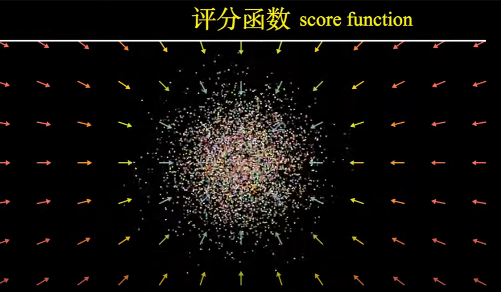
第三條路：這條路是以 score function (gradient of log-likelihood function) 為學習的 function.

Score function 其實是向量場函數，朝向 log-likelihood 更高的地方移動。 Neural network 就是在學這個函數。

(37) An artificial intelligence doctoral student tells you how the SORA diffusion model generates videos? - YouTube

Tweedie’s Formula: a Gaussian variable $\boldsymbol{z} \sim \mathcal{N}\left(\boldsymbol{z} ; \boldsymbol{\mu}_z, \boldsymbol{\Sigma}_z\right)$, Tweedie’s formula

\[\mathbb{E}\left[\boldsymbol{\mu}_z \mid \boldsymbol{z}\right]=\boldsymbol{z}+\boldsymbol{\Sigma}_z \nabla_{\boldsymbol{z}} \log p(\boldsymbol{z})\]

我們可以用 Tweedie’s formula 預測 true posterior mean of $\boldsymbol{x}t$ given its samples. $q\left(\boldsymbol{x}_t \mid \boldsymbol{x}_0\right)=\mathcal{N}\left(\boldsymbol{x}_t ; \sqrt{\bar{\alpha}_t} \boldsymbol{x}_0,\left(1-\bar{\alpha}_t\right) \mathbf{I}\right)$ 可以得到： $\mathbb{E}\left[\boldsymbol{\mu}_{x_t} \mid \boldsymbol{x}_t\right]=\boldsymbol{x}_t+\left(1-\bar{\alpha}_t\right) \nabla_{\boldsymbol{x}_t} \log p\left(\boldsymbol{x}_t\right)$ $\nabla{\boldsymbol{x}t} \log p(\boldsymbol{x}_t)$ 簡寫成 $\nabla \log p\left(\boldsymbol{x}_t\right)$ for notational simplicity. 根據 Tweedie’s formula, the best estimate for the true mean that $\boldsymbol{x}_t$ is generated from, $\boldsymbol{\mu}{x_t}=\sqrt{\bar{\alpha}_t} \boldsymbol{x}_0$, is defined as: $\begin{aligned} \sqrt{\bar{\alpha}_t} \boldsymbol{x}_0 &=\boldsymbol{x}_t+\left(1-\bar{\alpha}_t\right) \nabla \log p\left(\boldsymbol{x}_t\right) \\ \therefore \boldsymbol{x}_0 &=\frac{\boldsymbol{x}_t+\left(1-\bar{\alpha}_t\right) \nabla \log p\left(\boldsymbol{x}_t\right)}{\sqrt{\bar{\alpha}_t}} \end{aligned}$

再把上式代入 ground truth denoising transition mean $\eqref{MeanQ}$, 可以得到 $\begin{aligned} \boldsymbol{\mu}_q\left(\boldsymbol{x}_t, \boldsymbol{x}_0\right) &=\frac{\sqrt{\alpha_t}\left(1-\bar{\alpha}_{t-1}\right) \boldsymbol{x}_t+\sqrt{\bar{\alpha}_{t-1}}\left(1-\alpha_t\right) \boldsymbol{x}_0}{1-\bar{\alpha}_t} \\ &=\frac{1-\bar{\alpha}_t}{\left(1-\bar{\alpha}_t\right) \sqrt{\alpha_t}} \boldsymbol{x}_t+\frac{1-\alpha_t}{\sqrt{\alpha_t}} \nabla \log p\left(\boldsymbol{x}_t\right) \\ &=\frac{1}{\sqrt{\alpha_t}} \boldsymbol{x}_t+\frac{1-\alpha_t}{\sqrt{\alpha_t}} \nabla \log p\left(\boldsymbol{x}_t\right) \end{aligned}$ 因此我們也可以 use a neural network to approximate denoising transition mean $\boldsymbol{\mu}_{\boldsymbol{\theta}}\left(\boldsymbol{x}_t, t\right)$ as: $\boldsymbol{\mu}_{\boldsymbol{\theta}}\left(\boldsymbol{x}_t, t\right)=\frac{1}{\sqrt{\alpha_t}} \boldsymbol{x}_t+\frac{1-\alpha_t}{\sqrt{\alpha_t}} \boldsymbol{s}_{\boldsymbol{\theta}}\left(\boldsymbol{x}_t, t\right)$

如此對應的 optimization problem 變成：

$\underset{\boldsymbol{\theta}}{\arg \min } D_{\mathrm{KL}}\left(q\left(\boldsymbol{x}{t-1} \mid \boldsymbol{x}_t, \boldsymbol{x}_0\right) | p{\boldsymbol{\theta}}\left(\boldsymbol{x}{t-1} \mid \boldsymbol{x}_t\right)\right)$ $=\underset{\boldsymbol{\theta}}{\arg \min } D{\mathrm{KL}}\left(\mathcal{N}\left(\boldsymbol{x}{t-1} ; \boldsymbol{\mu}_q, \boldsymbol{\Sigma}_q(t)\right) | \mathcal{N}\left(\boldsymbol{x}{t-1} ; \boldsymbol{\mu}{\boldsymbol{\theta}}, \boldsymbol{\Sigma}_q(t)\right)\right)$ $=\underset{\boldsymbol{\theta}}{\arg \min } \frac{1}{2 \sigma_q^2(t)}\left[\left|\frac{1}{\sqrt{\alpha_t}} \boldsymbol{x}_t+\frac{1-\alpha_t}{\sqrt{\alpha_t}} \boldsymbol{s}{\boldsymbol{\theta}}\left(\boldsymbol{x}t, t\right)-\frac{1}{\sqrt{\alpha_t}} \boldsymbol{x}_t-\frac{1-\alpha_t}{\sqrt{\alpha_t}} \nabla \log p\left(\boldsymbol{x}_t\right)\right|_2^2\right]$ $=\underset{\boldsymbol{\theta}}{\arg \min } \frac{1}{2 \sigma_q^2(t)}\left[\left|\frac{1-\alpha_t}{\sqrt{\alpha_t}} \boldsymbol{s}{\boldsymbol{\theta}}\left(\boldsymbol{x}t, t\right)-\frac{1-\alpha_t}{\sqrt{\alpha_t}} \nabla \log p\left(\boldsymbol{x}_t\right)\right|_2^2\right]$ $=\underset{\boldsymbol{\theta}}{\arg \min } \frac{1}{2 \sigma_q^2(t)}\left[\left|\frac{1-\alpha_t}{\sqrt{\alpha_t}}\left(\boldsymbol{s}{\boldsymbol{\theta}}\left(\boldsymbol{x}t, t\right)-\nabla \log p\left(\boldsymbol{x}_t\right)\right)\right|_2^2\right]$ $=\underset{\boldsymbol{\theta}}{\arg \min } \frac{1}{2 \sigma_q^2(t)} \frac{\left(1-\alpha_t\right)^2}{\alpha_t}\left[\left|\boldsymbol{s}{\boldsymbol{\theta}}\left(\boldsymbol{x}_t, t\right)-\nabla \log p\left(\boldsymbol{x}_t\right)\right|_2^2\right]$

$\boldsymbol{s}_{\boldsymbol{\theta}}\left(\boldsymbol{x}_t, t\right)$ is a neural network $\theta$ that learns to predict the score function $\nabla \log p\left(\boldsymbol{x}_t\right)$, which is the gradient of $x_t$ in data space, for any arbitrary noise level $t$.

注意上式基本和 $\eqref{Noise}$ 非常像（只差了一個 scaling factor with time), 也就是 score function $\nabla \log p\left(\boldsymbol{x}_t\right)$ 非常類似 $\epsilon_0$ 的角色。我們可以用 Tweedie’s formula 得到這個 scaling factor. $\begin{aligned} \boldsymbol{x}_0=\frac{\boldsymbol{x}_t+\left(1-\bar{\alpha}_t\right) \nabla \log p\left(\boldsymbol{x}_t\right)}{\sqrt{\bar{\alpha}_t}} &=\frac{\boldsymbol{x}_t-\sqrt{1-\bar{\alpha}_t} \boldsymbol{\epsilon}_0}{\sqrt{\bar{\alpha}_t}} \\ \therefore\left(1-\bar{\alpha}_t\right) \nabla \log p\left(\boldsymbol{x}_t\right) &=-\sqrt{1-\bar{\alpha}_t} \boldsymbol{\epsilon}_0 \\ \nabla \log p\left(\boldsymbol{x}_t\right) &=-\frac{1}{\sqrt{1-\bar{\alpha}_t}} \boldsymbol{\epsilon}_0 \end{aligned}$ 所以學習 score function 其實和學習負的 noise 是一樣的意思 (up to a scaling factor). Score function 是 denoise.

三種 VDM 詮釋

Use neural network to learn original image from noisy image (denoise)
Use neural network to learn noise from diffusion noise (non-equilibrium diffusion)
Use neural network to learn the score function (gradient of log likelihood function) for arbitrary noise

對於通信或是信號處理專家，一般是萃取原始信號 (non-Gaussian)。學習 noise 聽起來像是一個頭痛的問題。事實上可以證明：無法從 additive white Gaussian noise (AIWG) 萃取出除了 mean (1st order), variance (2nd order) 以外的 (sufficient) statistics. 不過幸運的是 VDM 是 additive Gaussian noise but NOT white. ?

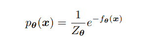
Enerrgy model looks like exponential family!!!!!!!!!!!!!!!

ML (Maximum likelihood) Estimator

$\theta_{MLE} = \arg_{\theta} \max p(x; \theta)$ 還是強調一下此處 $\theta$ 是 parameter, 不是 conditional distribution 中的 random variable.

Pros: (1) consistency, converges in probability to its true value; (2) almost unbiased; (3) 2nd order efficiency.

Cons: (1) point estimator, sensitive to assumption of distribution and parameter.

ML (Maximum Likelihood): 雙圓框的 $\mathbf{x}$ 是 observation or evidence. $\mathbf{x}$ 有一個 underlying distribution 是由一個 fixed and unknown parameter $\theta$ 決定。 $$數學是小學生程度 :)

EM (Expectation & Maximization?) Estimator –> extension of ML, 但是最重要概念是引入一個 hidden distribution!!!! Pave the way to Bayesian!

$\theta_{MLE} = \arg_{\theta} \max p(x; \theta)$ 還是強調一下此處 $\theta$ 是 parameter, 不是 conditional distribution 中的 random variable.

Pros: (1) consistency, converges in probability to its true value; (2) almost unbiased; (3) 2nd order efficiency.

Cons: (1) point estimator, sensitive to assumption of distribution and parameter.

ML (Maximum Likelihood): 雙圓框的 $\mathbf{x}$ 是 observation or evidence. $\mathbf{x}$ 有一個 underlying distribution 是由一個 fixed and unknown parameter $\theta$ 決定。 $$數學是小學生程度 :)

Bayesian Estimator –> extension of ML, 但是最重要概念是引入一個 hidden distribution!!!! Pave the way to Bayesian! $\theta$ becomes a distribution or a parameter for a hidden distribution! 連續改變 $\theta$ 就會得到一堆 distributions to approach x.

$\theta_{MLE} = \arg_{\theta} \max p(x; \theta)$ 還是強調一下此處 $\theta$ 是 parameter, 不是 conditional distribution 中的 random variable.

Pros: (1) consistency, converges in probability to its true value; (2) almost unbiased; (3) 2nd order efficiency.

Cons: (1) point estimator, sensitive to assumption of distribution and parameter.

ML (Maximum Likelihood): 雙圓框的 $\mathbf{x}$ 是 observation or evidence. $\mathbf{x}$ 有一個 underlying distribution 是由一個 fixed and unknown parameter $\theta$ 決定。 $$數學是小學生程度 :)

Prom: what if 並不存在這樣簡單的 parameter for a hidden distribution –> burden 變成如何找到這樣複雜 distribution!!

DLVM : $\theta$ from a parameter for a hidden distribution becomes a neural network mapping!!!!!!!!!!!!!!! 最大好處是 distribution very easy!!! normal distribution or uniform distribution!! 複雜的事留給 mapping using a learnable neural network!!!

$\theta_{MLE} = \arg_{\theta} \max p(x; \theta)$ 還是強調一下此處 $\theta$ 是 parameter, 不是 conditional distribution 中的 random variable.

Pros: (1) consistency, converges in probability to its true value; (2) almost unbiased; (3) 2nd order efficiency.

Cons: (1) point estimator, sensitive to assumption of distribution and parameter.

ML (Maximum Likelihood): 雙圓框的 $\mathbf{x}$ 是 observation or evidence. $\mathbf{x}$ 有一個 underlying distribution 是由一個 fixed and unknown parameter $\theta$ 決定。 $$數學是小學生程度 :)

VAE : Posterior distribution is untracble, 再引入另一個 (learnable) mapping 解決這個問題。

Probability/distributions 和 neural network 好像是天生一對！！

###

VAE 第一個 innovation (encoder+decoder): 使用 encoder neural network ($\phi$) 和 decoder neural network ($\theta$) 架構。從 autoencoder 的延伸似乎很直觀。但從 deterministic 延伸到 probabilistic 有點魔幻寫實，需要更嚴謹的數學框架。
VAE 第二個 innovation (DLVM): 引入 hidden (random) variable $\mathbf{z}$, 從 $\mathbf{z} \to \text{neural network}\,(\theta) \to \mathbf{x}.$ Hidden variable $\mathbf{z}$ 源自 (variational) EM + DAG; 再用 (deterministic) neural network of $\theta$ for parameter optimization. 這就是 DLVM (Deep Learning Variable Model) 的精神。 根據 (variational) EM:
- E-step: 找到 $q(\mathbf{z}) \approx p_{\theta}(\mathbf{z} \mid \mathbf{x})$, 也就是 posterior, 但我們知道在 DLVM posterior 是 intractable，必須用近似
- M-step: optimize $\theta$ based on posterior: $\underset{\boldsymbol{\theta}}{\operatorname{argmax}} E_{q(\mathbf{z})} \ln p_{\theta}(\mathbf{x}, \mathbf{z})$, 其中的 joint distribution 是 tractable, 但是 $q(\mathbf{z})$ intractable, 所以是卡在 posterior intractable 這個問題！
- Iterate E-step and M-step in (variational EM); 在 DLVM 就變成 SGD optimization!
VAE 第三個 innovation 就是為了解決2.的 posterior 問題 $q(\mathbf{z}) \to q_{\phi}(\mathbf{z}\mid x)$: 用另一個 (tractable) decoder neural network $\phi$, 來近似 (intractable) posterior $q_{\phi}(\mathbf{z}\mid x) \approx p(\mathbf{z}\mid x)$
- 因此 VAE 和 DLVM (or variational EM) 的差別在於 VAE 多了 decoder neural network $\phi$ ，所以三者的數學框架非常相似！
- VAE 的 training loss 包含 reconstruction loss (源自 encoder+decoder) + 上面的 M-step loss (源自 variational EM)
- Maximum likelihood optimization ~ minimum cross-entropy loss (not in this case) ~ M-step loss (in this case)
同樣的方法應該可以用在很多 DLVM 應用中。如果有 intractable posterior, 就用 (encoder) neural network 近似。但問題是要有方法 train 這個 encoder. VAE 很巧妙的同時 train encoder + decoder 是用原始的 image and generative image. 需要再檢驗。

下圖顯示 ML, EM, DLVM, VAE 的演進關係；DLVM 和 VAE echo 1-4. 雙圓框代表 observed random variable, 單圓框代表 hidden random variable. 單方框代表 (fixed and to be estimated) parameter.Diffusion Model is another generative model: VAE -> GAN -> Diffusion

[@luoUnderstandingDiffusion2022] shows

Diffusion model 可以視為 VAE 的延伸！

所以 diffusion model 和 VAE 的實際做法有什麼不同?

Appendix

Appendix A : DVM ELBO 推導

\[\begin{align*} \text{ELBO} &= \mathbb{E}_{q\left(\boldsymbol{x}_{1: T} \mid \boldsymbol{x}_0\right)}\left[\log \frac{p\left(\boldsymbol{x}_{0: T}\right)}{q\left(\boldsymbol{x}_{1: T} \mid \boldsymbol{x}_0\right)}\right]\\ &=\mathbb{E}_{q\left(\boldsymbol{x}_{1: T} \mid \boldsymbol{x}_0\right)}\left[\log \frac{p\left(\boldsymbol{x}_T\right) \prod_{t=1}^T p_{\boldsymbol{\theta}}\left(\boldsymbol{x}_{t-1} \mid \boldsymbol{x}_t\right)}{\prod_{t=1}^T q\left(\boldsymbol{x}_t \mid \boldsymbol{x}_{t-1}\right)}\right]\\ &=\mathbb{E}_{q\left(\boldsymbol{x}_{1: T} \mid \boldsymbol{x}_0\right)}\left[\log \frac{p\left(\boldsymbol{x}_T\right) p_{\boldsymbol{\theta}}\left(\boldsymbol{x}_0 \mid \boldsymbol{x}_1\right) \prod_{t=2}^T p_{\boldsymbol{\theta}}\left(\boldsymbol{x}_{t-1} \mid \boldsymbol{x}_t\right)}{q\left(\boldsymbol{x}_T \mid \boldsymbol{x}_{T-1}\right) \prod_{t=1}^{T-1} q\left(\boldsymbol{x}_t \mid \boldsymbol{x}_{t-1}\right)}\right]\\ &=\mathbb{E}_{q\left(\boldsymbol{x}_{1: T} \mid \boldsymbol{x}_0\right)}\left[\log \frac{p\left(\boldsymbol{x}_T\right) p_{\boldsymbol{\theta}}\left(\boldsymbol{x}_0 \mid \boldsymbol{x}_1\right) \prod_{t=1}^{T-1} p_{\boldsymbol{\theta}}\left(\boldsymbol{x}_t \mid \boldsymbol{x}_{t+1}\right)}{q\left(\boldsymbol{x}_T \mid \boldsymbol{x}_{T-1}\right) \prod_{t=1}^{T-1} q\left(\boldsymbol{x}_t \mid \boldsymbol{x}_{t-1}\right)}\right]\\ &=\mathbb{E}_{q\left(\boldsymbol{x}_{1: T} \mid \boldsymbol{x}_0\right)}\left[\log \frac{p\left(\boldsymbol{x}_T\right) p_{\boldsymbol{\theta}}\left(\boldsymbol{x}_0 \mid \boldsymbol{x}_1\right)}{q\left(\boldsymbol{x}_T \mid \boldsymbol{x}_{T-1}\right)}\right]+\mathbb{E}_{q\left(\boldsymbol{x}_{1: T} \mid \boldsymbol{x}_0\right)}\left[\log \prod_{t=1}^{T-1} \frac{p_{\boldsymbol{\theta}}\left(\boldsymbol{x}_t \mid \boldsymbol{x}_{t+1}\right)}{q\left(\boldsymbol{x}_t \mid \boldsymbol{x}_{t-1}\right)}\right]\\ &=\mathbb{E}_{q\left(\boldsymbol{x}_{1: T} \mid \boldsymbol{x}_0\right)}\left[\log p_{\boldsymbol{\theta}}\left(\boldsymbol{x}_0 \mid \boldsymbol{x}_1\right)\right]+\mathbb{E}_{q\left(\boldsymbol{x}_{1: T} \mid \boldsymbol{x}_0\right)}\left[\log \frac{p\left(\boldsymbol{x}_T\right)}{q\left(\boldsymbol{x}_T \mid \boldsymbol{x}_{T-1}\right)}\right]+\mathbb{E}_{q\left(\boldsymbol{x}_{1: T} \mid \boldsymbol{x}_0\right)}\left[\sum_{t=1}^{T-1} \log \frac{p_{\boldsymbol{\theta}}\left(\boldsymbol{x}_t \mid \boldsymbol{x}_{t+1}\right)}{q\left(\boldsymbol{x}_t \mid \boldsymbol{x}_{t-1}\right)}\right]\\ &=\mathbb{E}_{q\left(\boldsymbol{x}_{1: T} \mid \boldsymbol{x}_0\right)}\left[\log p_{\boldsymbol{\theta}}\left(\boldsymbol{x}_0 \mid \boldsymbol{x}_1\right)\right]+\mathbb{E}_{q\left(\boldsymbol{x}_{1: T} \mid \boldsymbol{x}_0\right)}\left[\log \frac{p\left(\boldsymbol{x}_T\right)}{q\left(\boldsymbol{x}_T \mid \boldsymbol{x}_{T-1}\right)}\right]+\sum_{t=1}^{T-1} \mathbb{E}_{q\left(\boldsymbol{x}_{1: T} \mid \boldsymbol{x}_0\right)}\left[\log \frac{p_{\boldsymbol{\theta}}\left(\boldsymbol{x}_t \mid \boldsymbol{x}_{t+1}\right)}{q\left(\boldsymbol{x}_t \mid \boldsymbol{x}_{t-1}\right)}\right]\\ &=\mathbb{E}_{q\left(\boldsymbol{x}_1 \mid \boldsymbol{x}_0\right)}\left[\log p_{\boldsymbol{\theta}}\left(\boldsymbol{x}_0 \mid \boldsymbol{x}_1\right)\right]+\mathbb{E}_{q\left(\boldsymbol{x}_{T-1}, \boldsymbol{x}_T \mid \boldsymbol{x}_0\right)}\left[\log \frac{p\left(\boldsymbol{x}_T\right)}{q\left(\boldsymbol{x}_T \mid \boldsymbol{x}_{T-1}\right)}\right]+\sum_{t=1}^{T-1} \mathbb{E}_{q\left(\boldsymbol{x}_{t-1}, \boldsymbol{x}_t, \boldsymbol{x}_{t+1} \mid \boldsymbol{x}_0\right)}\left[\log \frac{p_{\boldsymbol{\theta}}\left(\boldsymbol{x}_t \mid \boldsymbol{x}_{t+1}\right)}{q\left(\boldsymbol{x}_t \mid \boldsymbol{x}_{t-1}\right)}\right]\\ &=\underbrace{\mathbb{E}_{q\left(\boldsymbol{x}_1 \mid \boldsymbol{x}_0\right)}\left[\log p_\theta\left(\boldsymbol{x}_0 \mid \boldsymbol{x}_1\right)\right]}_{\text {reconstruction term }}-\underbrace{\mathbb{E}_{q\left(\boldsymbol{x}_{T-1} \mid \boldsymbol{x}_0\right)}\left[D_{\mathrm{KL}}\left(q\left(\boldsymbol{x}_T \mid \boldsymbol{x}_{T-1}\right) \| p\left(\boldsymbol{x}_T\right)\right)\right]}_{\text {prior matching term }}\\ &-\sum_{t=1}^{T-1} \underbrace{\mathbb{E}_{q\left(\boldsymbol{x}_{t-1}, \boldsymbol{x}_{t+1} \mid \boldsymbol{x}_0\right)}\left[D_{\mathrm{KL}}\left(q\left(\boldsymbol{x}_t \mid \boldsymbol{x}_{t-1}\right) \| p_\theta\left(\boldsymbol{x}_t \mid \boldsymbol{x}_{t+1}\right)\right)\right]}_{\text {consistency term }} \end{align*}\]

Appendix B : Conditional Distribution 推導

\[\begin{align*} &q\left(\boldsymbol{x}_{t-1} \mid \boldsymbol{x}_t, \boldsymbol{x}_0\right)=\frac{q\left(\boldsymbol{x}_t \mid \boldsymbol{x}_{t-1}, \boldsymbol{x}_0\right) q\left(\boldsymbol{x}_{t-1} \mid \boldsymbol{x}_0\right)}{q\left(\boldsymbol{x}_t \mid \boldsymbol{x}_0\right)}\\&=\frac{\mathcal{N}\left(\boldsymbol{x}_t ; \sqrt{\alpha_t} \boldsymbol{x}_{t-1},\left(1-\alpha_t\right) \mathbf{I}\right) \mathcal{N}\left(\boldsymbol{x}_{t-1} ; \sqrt{\bar{\alpha}_{t-1}} \boldsymbol{x}_0,\left(1-\bar{\alpha}_{t-1}\right) \mathbf{I}\right)}{\mathcal{N}\left(\boldsymbol{x}_t ; \sqrt{\bar{\alpha}_t} \boldsymbol{x}_0,\left(1-\bar{\alpha}_t\right) \mathbf{I}\right)}\\&\propto \exp \left\{-\left[\frac{\left(\boldsymbol{x}_t-\sqrt{\alpha_t} \boldsymbol{x}_{t-1}\right)^2}{2\left(1-\alpha_t\right)}+\frac{\left(\boldsymbol{x}_{t-1}-\sqrt{\bar{\alpha}_{t-1}} \boldsymbol{x}_0\right)^2}{2\left(1-\bar{\alpha}_{t-1}\right)}-\frac{\left(\boldsymbol{x}_t-\sqrt{\bar{\alpha}_t} \boldsymbol{x}_0\right)^2}{2\left(1-\bar{\alpha}_t\right)}\right]\right\}\\&=\exp \left\{-\frac{1}{2}\left[\frac{\left(\boldsymbol{x}_t-\sqrt{\alpha_t} \boldsymbol{x}_{t-1}\right)^2}{1-\alpha_t}+\frac{\left(\boldsymbol{x}_{t-1}-\sqrt{\bar{\alpha}_{t-1}} \boldsymbol{x}_0\right)^2}{1-\bar{\alpha}_{t-1}}-\frac{\left(\boldsymbol{x}_t-\sqrt{\bar{\alpha}_t} \boldsymbol{x}_0\right)^2}{1-\bar{\alpha}_t}\right]\right\}\\&=\exp \left\{-\frac{1}{2}\left[\frac{\left(-2 \sqrt{\alpha_t} \boldsymbol{x}_t \boldsymbol{x}_{t-1}+\alpha_t \boldsymbol{x}_{t-1}^2\right)}{1-\alpha_t}+\frac{\left(\boldsymbol{x}_{t-1}^2-2 \sqrt{\bar{\alpha}_{t-1}} \boldsymbol{x}_{t-1} \boldsymbol{x}_0\right)}{1-\bar{\alpha}_{t-1}}+C\left(\boldsymbol{x}_t, \boldsymbol{x}_0\right)\right]\right\}\\&\propto \exp \left\{-\frac{1}{2}\left[-\frac{2 \sqrt{\alpha_t} \boldsymbol{x}_t \boldsymbol{x}_{t-1}}{1-\alpha_t}+\frac{\alpha_t \boldsymbol{x}_{t-1}^2}{1-\alpha_t}+\frac{\boldsymbol{x}_{t-1}^2}{1-\bar{\alpha}_{t-1}}-\frac{2 \sqrt{\alpha_{t-1}} \boldsymbol{x}_{t-1} \boldsymbol{x}_0}{1-\bar{\alpha}_{t-1}}\right]\right\}\\&=\exp \left\{-\frac{1}{2}\left[\left(\frac{\alpha_t}{1-\alpha_t}+\frac{1}{1-\bar{\alpha}_{t-1}}\right) \boldsymbol{x}_{t-1}^2-2\left(\frac{\sqrt{\alpha_t} \boldsymbol{x}_t}{1-\alpha_t}+\frac{\sqrt{\bar{\alpha}_{t-1}} \boldsymbol{x}_0}{1-\bar{\alpha}_{t-1}}\right) \boldsymbol{x}_{t-1}\right]\right\}\\&=\exp \left\{-\frac{1}{2}\left[\frac{\alpha_t\left(1-\bar{\alpha}_{t-1}\right)+1-\alpha_t}{\left(1-\alpha_t\right)\left(1-\bar{\alpha}_{t-1}\right)} \boldsymbol{x}_{t-1}^2-2\left(\frac{\sqrt{\alpha_t} \boldsymbol{x}_t}{1-\alpha_t}+\frac{\sqrt{\bar{\alpha}_{t-1}} \boldsymbol{x}_0}{1-\bar{\alpha}_{t-1}}\right) \boldsymbol{x}_{t-1}\right]\right\}\\&=\exp \left\{-\frac{1}{2}\left[\frac{\alpha_t-\bar{\alpha}_t+1-\alpha_t}{\left(1-\alpha_t\right)\left(1-\bar{\alpha}_{t-1}\right)} \boldsymbol{x}_{t-1}^2-2\left(\frac{\sqrt{\alpha_t} \boldsymbol{x}_t}{1-\alpha_t}+\frac{\sqrt{\bar{\alpha}_{t-1}} \boldsymbol{x}_0}{1-\bar{\alpha}_{t-1}}\right) \boldsymbol{x}_{t-1}\right]\right\}\\&=\exp \left\{-\frac{1}{2}\left[\frac{1-\bar{\alpha}_t}{\left(1-\alpha_t\right)\left(1-\bar{\alpha}_{t-1}\right)} \boldsymbol{x}_{t-1}^2-2\left(\frac{\sqrt{\alpha_t} \boldsymbol{x}_t}{1-\alpha_t}+\frac{\sqrt{\alpha_{t-1}} \boldsymbol{x}_0}{1-\bar{\alpha}_{t-1}}\right) \boldsymbol{x}_{t-1}\right]\right\}\\&=\exp \left\{-\frac{1}{2}\left(\frac{1-\bar{\alpha}_t}{\left(1-\alpha_t\right)\left(1-\bar{\alpha}_{t-1}\right)}\right)\left[\boldsymbol{x}_{t-1}^2-2 \frac{\left(\frac{\sqrt{\alpha_t} x_t}{1-\alpha_t}+\frac{\sqrt{\bar{\alpha}_{t-1}} \boldsymbol{x}_0}{1-\bar{\alpha}_{t-1}}\right)}{\frac{1-\bar{\alpha}_t}{\left(1-\bar{\alpha}_t\right)\left(1-\bar{\alpha}_{t-1}\right)}} \boldsymbol{x}_{t-1}\right]\right\}\\&=\exp \left\{-\frac{1}{2}\left(\frac{1-\bar{\alpha}_t}{\left(1-\alpha_t\right)\left(1-\bar{\alpha}_{t-1}\right)}\right)\left[\boldsymbol{x}_{t-1}^2-2 \frac{\left(\frac{\sqrt{\alpha_t} \boldsymbol{x}_t}{1-\alpha_t}+\frac{\sqrt{\bar{\alpha}_{t-1}} \boldsymbol{x}_0}{1-\bar{\alpha}_{t-1}}\right)\left(1-\alpha_t\right)\left(1-\bar{\alpha}_{t-1}\right)}{1-\bar{\alpha}_t} \boldsymbol{x}_{t-1}\right]\right\}\\&=\exp \left\{-\frac{1}{2}\left(\frac{1}{\frac{\left(1-\alpha_t\right)\left(1-\bar{\alpha}_{t-1}\right)}{1-\bar{\alpha}_t}}\right)\left[\boldsymbol{x}_{t-1}^2-2 \frac{\sqrt{\alpha_t}\left(1-\bar{\alpha}_{t-1}\right) \boldsymbol{x}_t+\sqrt{\bar{\alpha}_{t-1}}\left(1-\alpha_t\right) \boldsymbol{x}_0}{1-\bar{\alpha}_t} \boldsymbol{x}_{t-1}\right]\right\}\\&\propto \mathcal{N}(\boldsymbol{x}_{t-1} ; \underbrace{\frac{\sqrt{\alpha_t}\left(1-\bar{\alpha}_{t-1}\right) \boldsymbol{x}_t+\sqrt{\bar{\alpha}_{t-1}}\left(1-\alpha_t\right) \boldsymbol{x}_0}{1-\bar{\alpha}_t}}_{\mu_q\left(\boldsymbol{x}_t, \boldsymbol{x}_0\right)}, \underbrace{\left.\frac{\left(1-\alpha_t\right)\left(1-\bar{\alpha}_{t-1}\right)}{1-\bar{\alpha}_t} \mathbf{I}\right)}_{\boldsymbol{\Sigma}_q(t)} \end{align*}\]

Appendix C : KL Divergence

\[\begin{align*} &\underset{\boldsymbol{\theta}}{\arg \min } D_{\mathrm{KL}}\left(q\left(\boldsymbol{x}_{t-1} \mid \boldsymbol{x}_t, \boldsymbol{x}_0\right) \| p_{\boldsymbol{\theta}}\left(\boldsymbol{x}_{t-1} \mid \boldsymbol{x}_t\right)\right)\\=& \underset{\boldsymbol{\theta}}{\arg \min } D_{\mathrm{KL}}\left(\mathcal{N}\left(\boldsymbol{x}_{t-1} ; \boldsymbol{\mu}_q, \boldsymbol{\Sigma}_q(t)\right) \| \mathcal{N}\left(\boldsymbol{x}_{t-1} ; \boldsymbol{\mu}_{\boldsymbol{\theta}}, \boldsymbol{\Sigma}_q(t)\right)\right)\\=& \underset{\boldsymbol{\theta}}{\arg \min } \frac{1}{2 \sigma_q^2(t)}\left[\left\|\frac{\sqrt{\alpha_t}\left(1-\bar{\alpha}_{t-1}\right) \boldsymbol{x}_t+\sqrt{\bar{\alpha}_{t-1}}\left(1-\alpha_t\right) \hat{\boldsymbol{x}}_{\boldsymbol{\theta}}\left(\boldsymbol{x}_t, t\right)}{1-\bar{\alpha}_t}-\frac{\sqrt{\alpha_t}\left(1-\bar{\alpha}_{t-1}\right) \boldsymbol{x}_t+\sqrt{\bar{\alpha}_{t-1}}\left(1-\alpha_t\right) \boldsymbol{x}_0}{1-\bar{\alpha}_t}\right\|_2^2\right]\\=& \underset{\boldsymbol{\theta}}{\arg \min } \frac{1}{2 \sigma_q^2(t)}\left[\left\|\frac{\sqrt{\bar{\alpha}_{t-1}}\left(1-\alpha_t\right) \hat{\boldsymbol{x}}_{\boldsymbol{\theta}}\left(\boldsymbol{x}_t, t\right)}{1-\bar{\alpha}_t}-\frac{\sqrt{\bar{\alpha}_{t-1}}\left(1-\alpha_t\right) \boldsymbol{x}_0}{1-\bar{\alpha}_t}\right\|_2^2\right]\\=& \underset{\boldsymbol{\theta}}{\arg \min } \frac{1}{2 \sigma_q^2(t)}\left[\left\|\frac{\sqrt{\bar{\alpha}_{t-1}}\left(1-\alpha_t\right)}{1-\bar{\alpha}_t}\left(\hat{\boldsymbol{x}}_{\boldsymbol{\theta}}\left(\boldsymbol{x}_t, t\right)-\boldsymbol{x}_0\right)\right\|_2^2\right]\\=& \underset{\boldsymbol{\theta}}{\arg \min } \frac{1}{2 \sigma_q^2(t)} \frac{\bar{\alpha}_{t-1}\left(1-\alpha_t\right)^2}{\left(1-\bar{\alpha}_t\right)^2}\left[\left\|\hat{\boldsymbol{x}}_{\boldsymbol{\theta}}\left(\boldsymbol{x}_t, t\right)-\boldsymbol{x}_0\right\|_2^2\right] \end{align*}\]

Appendix D : Denoise 推導

\[\begin{aligned} &\frac{1}{2 \sigma_q^2(t)} \frac{\bar{\alpha}_{t-1}\left(1-\alpha_t\right)^2}{\left(1-\bar{\alpha}_t\right)^2}\left[\left\|\hat{\boldsymbol{x}}_{\boldsymbol{\theta}}\left(\boldsymbol{x}_t, t\right)-\boldsymbol{x}_0\right\|_2^2\right]\\ =&\frac{1}{2 \frac{\left(1-\alpha_t\right)\left(1-\bar{\alpha}_{t-1}\right)}{1-\bar{\alpha}_t}} \frac{\bar{\alpha}_{t-1}\left(1-\alpha_t\right)^2}{\left(1-\bar{\alpha}_t\right)^2}\left[\left\|\hat{\boldsymbol{x}}_{\boldsymbol{\theta}}\left(\boldsymbol{x}_t, t\right)-\boldsymbol{x}_0\right\|_2^2\right]\\ =&\frac{1}{2} \frac{1-\bar{\alpha}_t}{\left(1-\alpha_t\right)\left(1-\bar{\alpha}_{t-1}\right)} \frac{\bar{\alpha}_{t-1}\left(1-\alpha_t\right)^2}{\left(1-\bar{\alpha}_t\right)^2}\left[\left\|\hat{\boldsymbol{x}}_{\boldsymbol{\theta}}\left(\boldsymbol{x}_t, t\right)-\boldsymbol{x}_0\right\|_2^2\right]\\ =&\frac{1}{2} \frac{\bar{\alpha}_{t-1}\left(1-\alpha_t\right)}{\left(1-\bar{\alpha}_{t-1}\right)\left(1-\bar{\alpha}_t\right)}\left[\left\|\hat{\boldsymbol{x}}_{\boldsymbol{\theta}}\left(\boldsymbol{x}_t, t\right)-\boldsymbol{x}_0\right\|_2^2\right]\\ =&\frac{1}{2} \frac{\bar{\alpha}_{t-1}-\bar{\alpha}_t}{\left(1-\bar{\alpha}_{t-1}\right)\left(1-\bar{\alpha}_t\right)}\left[\left\|\hat{\boldsymbol{x}}_{\boldsymbol{\theta}}\left(\boldsymbol{x}_t, t\right)-\boldsymbol{x}_0\right\|_2^2\right]\\ =&\frac{1}{2} \frac{\bar{\alpha}_{t-1}-\bar{\alpha}_{t-1} \bar{\alpha}_t+\bar{\alpha}_{t-1} \bar{\alpha}_t-\bar{\alpha}_t}{\left(1-\bar{\alpha}_{t-1}\right)\left(1-\bar{\alpha}_t\right)}\left[\left\|\hat{\boldsymbol{x}}_{\boldsymbol{\theta}}\left(\boldsymbol{x}_t, t\right)-\boldsymbol{x}_0\right\|_2^2\right]\\ =&\frac{1}{2} \frac{\bar{\alpha}_{t-1}\left(1-\bar{\alpha}_t\right)-\bar{\alpha}_t\left(1-\bar{\alpha}_{t-1}\right)}{\left(1-\bar{\alpha}_{t-1}\right)\left(1-\bar{\alpha}_t\right)}\left[\left\|\hat{\boldsymbol{x}}_{\boldsymbol{\theta}}\left(\boldsymbol{x}_t, t\right)-\boldsymbol{x}_0\right\|_2^2\right]\\ =&\frac{1}{2}\left(\frac{\bar{\alpha}_{t-1}\left(1-\bar{\alpha}_t\right)}{\left(1-\bar{\alpha}_{t-1}\right)\left(1-\bar{\alpha}_t\right)}-\frac{\bar{\alpha}_t\left(1-\bar{\alpha}_{t-1}\right)}{\left(1-\bar{\alpha}_{t-1}\right)\left(1-\bar{\alpha}_t\right)}\right)\left[\left\|\hat{\boldsymbol{x}}_{\boldsymbol{\theta}}\left(\boldsymbol{x}_t, t\right)-\boldsymbol{x}_0\right\|_2^2\right]\\ =&\frac{1}{2}\left(\frac{\bar{\alpha}_{t-1}}{1-\bar{\alpha}_{t-1}}-\frac{\bar{\alpha}_t}{1-\bar{\alpha}_t}\right)\left[\left\|\hat{x}_{\boldsymbol{\theta}}\left(\boldsymbol{x}_t, t\right)-\boldsymbol{x}_0\right\|_2^2\right]\\ \end{aligned}\]

Appendix D : Denoising Transition Mean 推導

\[\begin{aligned} \boldsymbol{\mu}_q\left(\boldsymbol{x}_t, \boldsymbol{x}_0\right) &=\frac{\sqrt{\alpha_t}\left(1-\bar{\alpha}_{t-1}\right) \boldsymbol{x}_t+\sqrt{\bar{\alpha}_{t-1}}\left(1-\alpha_t\right) \boldsymbol{x}_0}{1-\bar{\alpha}_t} \\ &=\frac{\sqrt{\alpha_t}\left(1-\bar{\alpha}_{t-1}\right) \boldsymbol{x}_t+\sqrt{\bar{\alpha}_{t-1}}\left(1-\alpha_t\right) \frac{\boldsymbol{x}_t+\left(1-\bar{\alpha}_t\right) \nabla \log p\left(\boldsymbol{x}_t\right)}{\sqrt{\alpha_t}}}{1-\bar{\alpha}_t} \\ &=\frac{\sqrt{\alpha_t}\left(1-\bar{\alpha}_{t-1}\right) \boldsymbol{x}_t+\left(1-\alpha_t\right) \frac{\boldsymbol{x}_t+\left(1-\bar{\alpha}_t\right) \nabla \log p\left(\boldsymbol{x}_t\right)}{\sqrt{\alpha_t}}}{1-\bar{\alpha}_t} \\ &=\frac{\sqrt{\alpha_t}\left(1-\bar{\alpha}_{t-1}\right) \boldsymbol{x}_t}{1-\bar{\alpha}_t}+\frac{\left(1-\alpha_t\right) \boldsymbol{x}_t}{\left(1-\bar{\alpha}_t\right) \sqrt{\alpha_t}}+\frac{\left(1-\alpha_t\right)\left(1-\bar{\alpha}_t\right) \nabla \log p\left(\boldsymbol{x}_t\right)}{\left(1-\bar{\alpha}_t\right) \sqrt{\alpha_t}} \\ &=\left(\frac{\sqrt{\alpha_t}\left(1-\bar{\alpha}_{t-1}\right)}{1-\bar{\alpha}_t}+\frac{1-\alpha_t}{\left(1-\bar{\alpha}_t\right) \sqrt{\alpha_t}}\right) \boldsymbol{x}_t+\frac{1-\alpha_t}{\sqrt{\alpha_t}} \nabla \log p\left(\boldsymbol{x}_t\right) \\ &=\left(\frac{\alpha_t\left(1-\bar{\alpha}_{t-1}\right)}{\left(1-\bar{\alpha}_t\right) \sqrt{\alpha_t}}+\frac{1-\alpha_t}{\left(1-\bar{\alpha}_t\right) \sqrt{\alpha_t}}\right) \boldsymbol{x}_t+\frac{1-\alpha_t}{\sqrt{\alpha_t}} \nabla \log p\left(\boldsymbol{x}_t\right) \\ &=\frac{\alpha_t-\bar{\alpha}_t+1-\alpha_t}{\left(1-\bar{\alpha}_t\right) \sqrt{\alpha_t}} \boldsymbol{x}_t+\frac{1-\alpha_t}{\sqrt{\alpha_t}} \nabla \log p\left(\boldsymbol{x}_t\right) \\ &=\frac{1-\bar{\alpha}_t}{\left(1-\bar{\alpha}_t\right) \sqrt{\alpha_t}} \boldsymbol{x}_t+\frac{1-\alpha_t}{\sqrt{\alpha_t}} \nabla \log p\left(\boldsymbol{x}_t\right) \\ &=\frac{1}{\sqrt{\alpha_t}} \boldsymbol{x}_t+\frac{1-\alpha_t}{\sqrt{\alpha_t}} \nabla \log p\left(\boldsymbol{x}_t\right) \end{aligned}\]

[@kingmaIntroductionVariational2019] : excellent reference for VAE [@escuderoVariationalAutoEncoders2020] : very good article for VAE

Reference

Escudero, Mauro Camara. 2020. “Variational Auto-Encoders and the Expectation-Maximization Algorithm.” Mauro Camara Escudero. July 15, 2020. https://maurocamaraescudero.netlify.app/post/variational-auto-encoders-and-the-expectation-maximization-algorithm/.

Kingma, Diederik P., and Max Welling. 2019. “An Introduction to Variational Autoencoders.” Foundations and Trends in Machine Learning12 (4): 307–92. https://doi.org/10.1561/2200000056.

Luo, Calvin. 2022. “Understanding Diffusion Models: A Unified Perspective.” arXiv. https://doi.org/10.48550/arXiv.2208.11970.

See Appendix A for derivation. ↩