Computer Vision - UNet from Autoencoder and FCN

UNet 可視為 Autoencoder 的一種變形，因為它的模型結構類似U型而得名。或是視為 FCN 的對稱改良版。

UNet 的 key ingredient: (1) 對稱的 encoder + decoder (from autoencoder); (2) bottleneck layer (from FCN); (3) (long) skip link from encoder to decoder (from FCN).

Improvement from UNet: (1) Add mixed long and short skip links; (2) Add more down-up sampling network

UNet 前世今生一：Autoencoder

Autoencoder 包含 encoder and decoder. Encoder 常常用來作爲 feature extract at low dimenstion. Decoder 剛好相反是升維，不過需要搭配 variational 手法 in training, i.e. variational autoencoder, 用於 image generation (e.g. MNIST number generation)

完整的 autoencoder, encoder+decoder, 是否有其他用途？答案是肯定的，可以用於 pixel-level image or video processing, 例如 segmentation, denoise, deblur, dehaze, etc.

Autoencoder 的主要問題是 quality. 在 encoder 降維做 feature extraction 的過程中，會丟失一些細節，只留下比較 high level information (e.g. object level feature)。之後的 decoder 從低維 upsampling 到高維的 image，可以視爲一種 filtering, 因爲缺乏細節，有可能會讓 output image 變得模糊。

很自然的想法就是提供高維的 skip link, 不至於讓高維的 information 在 decoder 降維都丟失。這就是 U-Net 的精神。

UNet 前世今生二：Fully Convolutional Network (FCN)

注意這裏 FCN 不是 fully connected network, 而是 fully convolutional network.

What and Why FCN?

对于一般的分类CNN网络，如VGG和Resnet，都会在网络的最后加入一些 (不止一層) 全连接层 (fully-connected layer, 如下圖 Hidden Layer H)，经过softmax后就可以获得 class probability.

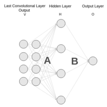
但是这个 probability information 是 1D 的，即只能标识整个图片的类别，不能标识每个像素点的类别。如下圖的 (a) 的 1D 4096/4096/1000 fully-connected layers. 所以这种全连接方法不适用于图像分割

而 FCN 提出可以把后面几个全连接 (fully connected layers) 都换成卷积 (convolutionalization), i.e. fully-connnected 1D 4096/4096/1000 layers 換成 convolutioned 2D 4095/4096/1000 layers. [longFullyConvolutional2015] 这样就可以获得一张 2D 的 feature map，后接softmax获得每个像素点的分类信息 (2D heat map)，从而解决了分割问题，如下图 (b).

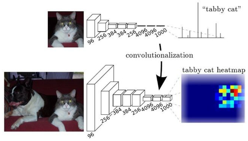
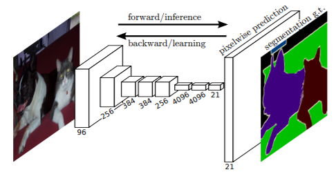
上面的缺點也很明顯，就是 2D heat map 的細緻度 (granularity) 不足。解決的方法就是用 up-sampling 得到 pixel-level 2D heat map 如下圖。

FCN Up-Sampling

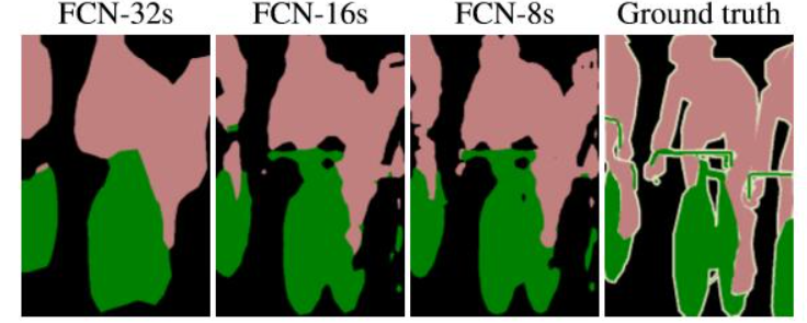
FCN 使用的 up-sampling 如下圖。FCN paper 試了幾種 upsampling 的方法:

直接把 pool5 (down-sampling by 32) up-sampling x32, 稱爲 FCN-32s;
Pool5 先 up-sampling x2, 再和 pool4 相加，再 up-sampling x16, 稱爲 FCN-16s;
把前面相加的結果再 up-sampling x2, 再和 pool3 相加，再 up-sampling x8, 稱爲 FCN-8s.

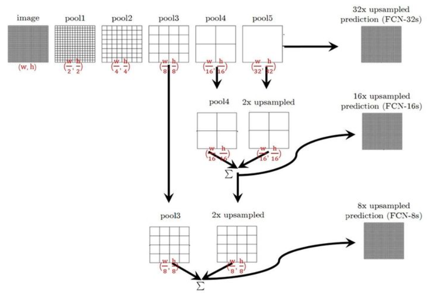
結果大概可以猜出來， FCN-8s > FCN-16s > FCN-32s, 如下圖。FCN-8s 最重要的 innovation 就是 shortcut from encoder to decoder, 這是之後 UNet 的濫殤。不確定 FCN 爲什麽不繼續做 FCN-4s or FCN-2s or FCN-s, 是結果沒有顯著的改善，還是其他的原因。

UNet 引入 shortcut 的觀念，同時又有點不同：

Up-sampling 和 short-cut 的結合在UNet 是用 concate，在 FCN 卻是相加。
UNet encoder 和 decoder 是對稱的，每一層都有 shortcut from encoder to decoder.
是不是因爲 UNet 使用 concate 才能 enable all layer shortcut? TBC.

最後還有一個 trick, 有兩種 up-sampling 方法

Resize: use interpolation (e.g. bilinear or bicubic or bi???), 見另文。可視為 deconvolution 的 special case (fixed coefficient filter)
Deconvolution or Transposed Convolution

UNet 結構

UNet 可視為 Autoencoder 的一種變形，因為它的模型結構類似U型而得名。或是視為 FCN 的對稱改良版。如下圖。

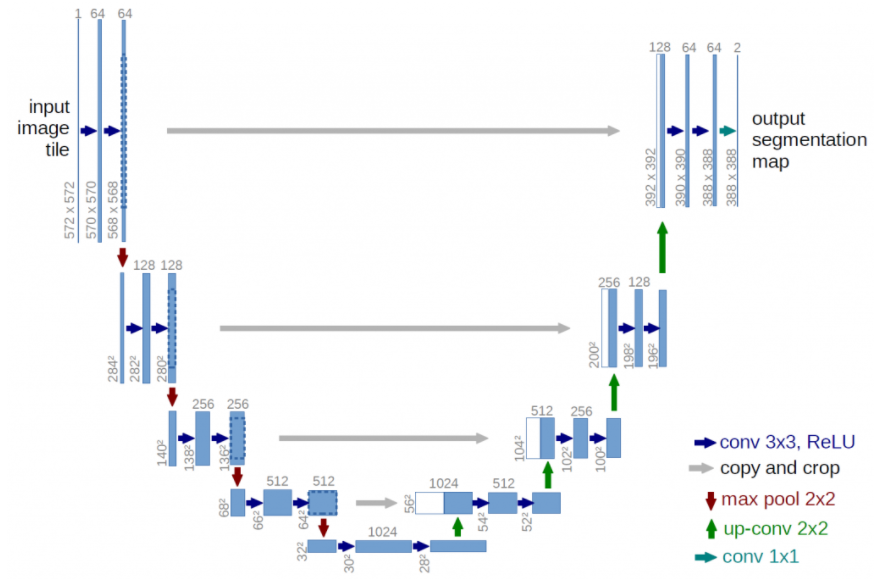
U-Net 架構分分爲三個部分：(1) contraction (降維，類似 encoder)；(2) bottleneck (from FCN, 見下文); (3) expansion (升維，類似 decoder)：

Contraction: many blocks, each block 包含兩個 3x3 convolution layers followed by a 2x2 max pooling. The number of kernels or feature maps after layer dimension reduction 加倍。目的是學習 high level features. Contraction 部分和一般 CNN network 非常類似或是一樣, e.g. VGG, or auto-encoder 的 encoder.
Expansion: 這是 U-Net 的核心部分。
- 基本的結構就是 reverse contraction 部分：each block 包含兩個 3x3 convolution layers followd by a 2x2 up-sampling layer. Feature maps or kernels after layer dimension expansion 減半。
- 重點：每個 block input 有兩個 inputs, 一個來自 up-sampling layer, 另一個來自對應的 encoder feature map, 兩者 equal size tensor concatenate. 這樣可以保證在 reconstruct output image 學到 encoder low level and high level feature maps. 我們把這種橫向的 connection 稱爲 short-cut.
Add short-cut from encoder to decoder. 這非常重要！如果沒有 short-cut 基本就是 autoencoder.
在變形的 U-Net, short-cut 並不限制在同一個 level from encoder-to-decoder. 可以有 encoder-to-encoder, 或是 decoder-to-decoder 長的或是短的 short-cut.
U-Net 基本變成影像處理網絡的 backbone and baseline, e.g. image segmentation, denoise, deblur, super resolution, HDR (high dynamic range), etc.
完整的 UNet 的參數有 xxx M 個，算力需求是 xx GOPs.

U-Net Rationale

基於 CNN 的網絡背後的主要想法是學習 feature map of an image, i.e. encoder. 這對image 分類問題效果很好，因為 image 先被轉換為 (one-dimension) vector，再進一步用於分類。 [sankesaraUNet2019]

但是在image 分割中，我們不僅需要將 feature map 轉換為 1D vector ，還需要從該 vector 重建 image, i.e. decoder. 這是一項艱鉅的任務，因為將 vector 轉換為 image (decoder) 比將 image 轉換為 vector (encoder) 要困難得多。 UNet 的整個想法就是圍繞這個問題展開的。

在將 image 轉換為 vector (encoder) 時，我們已經學習了 image 的 feature map，所以為什麼不使用相同的 mapping 將其再次轉換為 image。這是 UNet 背後的秘訣。

Use the same feature maps that are used for contraction to expand a vector to a segmented image. 這將保持 image 的結構完整性，從而極大地減少失真。

簡單說就是把 encoder 降維過程的 feature maps (包含 low level 的 feature) forward 到 decoder 融合到升維過程。

這是 pixel-level image task (e.g. segmentation, super resolution) 和 object-level image task (e.g. classification, detection) 本質上的不同。

UNet 結構改良

「从UNet的网络结构我们会发现两个最主要的特点，一个是它的U型结构，一个是它的跳层连接。」 其中UNet的编码器一共有4次下采样来获取高级语义信息，解码器自然对应了4次上采样来进行分辨率恢复，为了减少下采样过程带来的空间信息损失跳层连接被引入了，通过Concat的方式使得上采样恢复的特征图中包含更多low-level的语义信息，使得结果的精细程度更好。

使用转置卷积的UNet参数量是31M左右，如果对其channel进行缩小例如缩小两倍，参数量可以变为7.75M左右，缩小4倍变成2M左右，可以说是非常的轻量级了。UNet不仅仅在医学分割中被大量应用，也在工业界发挥了很大的作用。

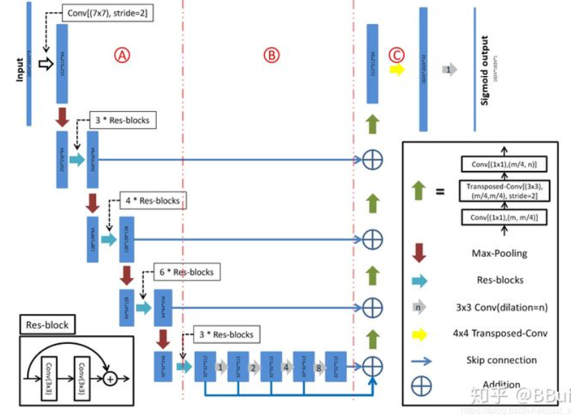
我们知道UNet做下采样的BackNone是普通的CBR模块(Conv+BN+ReLU)堆叠的，一个自然的想法就是如果将学习更强的ResNet当作UNet的BackBone效果是否会更好呢？ CVPR 2017的LinkNet给出了答案。LinkNet的网络结构如下所示：

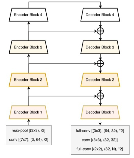
Encoder block (with residue link) and decoder block

其中，conv 代表卷积，full-conv 代表全卷积 (fully convolutional?)，/2代表 down sampling 的 stride 是2，*2代表 up sampling 的因子是2。在卷积层之后添加 BN，后加 ReLU。左半部分表示编码，右半部分表示解码。编码块基于ResNet18。

这项工作的主要贡献是在原始的UNet 的 encoder 引入了 residue or short skip link，并直接将编码器与解码器连接 (short-cut or long skip link) 来提高准确率，其實這也可以視爲是一種 residue link? 一定程度上减少了处理时间。通过这种方式，保留编码部分中不同层丢失的信息，同时，在进行重新学习丢失的信息时并未增加额外的参数与操作。在Citycapes 和 CamVID 数据集上的实验结果证明残差连接的引入（LinkNet without skip）使得mIOU获得了提升。

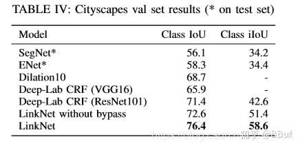
这篇论文的主要提升技巧在于它的 skip 技巧，但我们也可以看到ResNet也进一步对网络的效果带来了改善，所以至少说明ResNet是可以当成BackBone应用在UNet的，这样结果至少不会差。

Local shortcut: D-LinkNet

CVPR 2018北邮在DeepGlobe Road Extraction Challenge全球卫星图像道路提取）比赛中勇夺冠军，他们提出了一个新网络名为D-LinkNet，论文链接以及代码/PPT见附录。

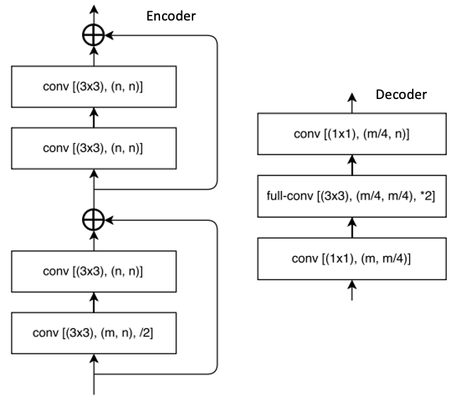
D-LinkNet使用LinkNet作为基本骨架，使用在ImageNet数据集上与训练好的ResNet作为网络的encoder，并在中心部分添加带有shortcut的dilated-convolution层，使得整个网络识别能力更强、接收域更大、融合多尺度信息。网络中心部分展开示意图如下：

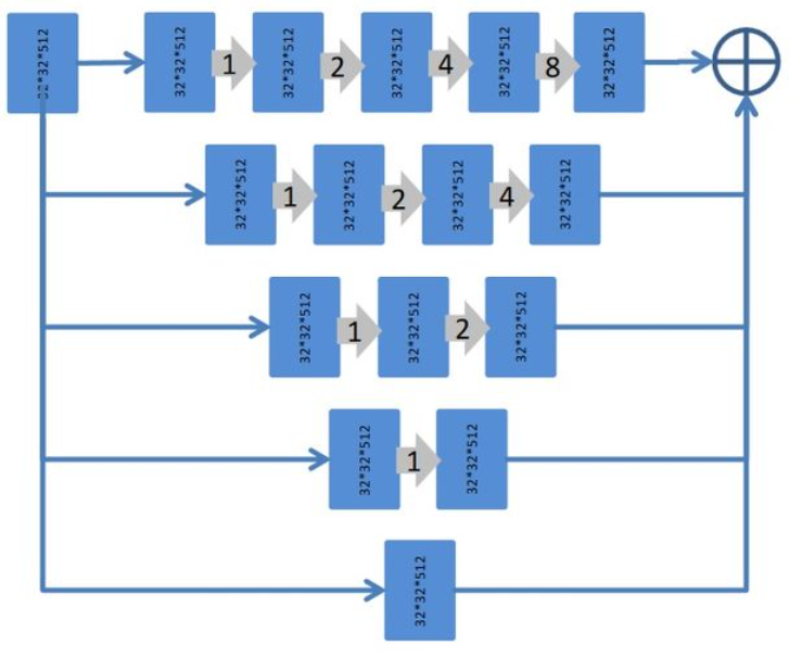
这篇论文和ResNet的关系实际上和LinkNet表达出的意思一致，就是大量增加 short or long skip links 並将其应用在BackBone部分增强特征表达能力。

Mixed Long and Short Skip Links

这篇文章其实是比上两篇文章早的，但我想放到最后这个位置来谈一下，这篇文章是DLMIA 2016的文章，名为：「The Importance of Skip Connections in Biomedical Image Segmentation」 。这一网络结构如下图所示，对图的解释来自akkaze-郑安坤的文章

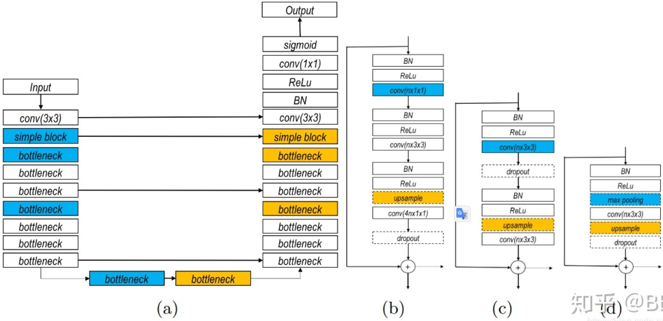
(a) 整个网络结构

使用下采样（蓝色）：这是一条收缩路径。

上采样（黄色）：这是一条不断扩大的路径。

这是一个类似于U-Net的FCN架构。

并且从收缩路径到扩展路径之间存在很长的跳过连接。

（b）瓶颈区

使用 $1×1Conv-3×3Conv-1×1Conv$ ，因此称为瓶颈。它已在ResNet中使用。

在每次转化前都使用 $BN-ReLU$ ，这是激活前ResNet的想法。

（c）基本块

两个 $3×3$ 卷积，它也用在ResNet中。

（d）简单块

$1$ 个 $3×3$ 卷积

（b）-（d）

所有块均包含短跳转连接。

下面的Table1表示整个网络的维度变化：

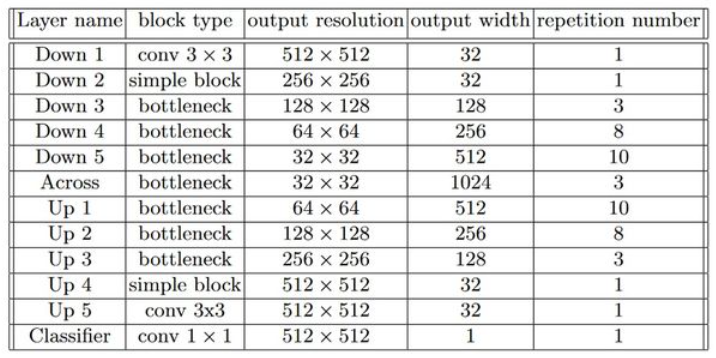
接下来是这节要分析的重点了，也就是长短跳过网络中两种不同类型的跳跃连接究竟对UNet的结果参生了什么影响？

这里训练集以 $30$ 张电子显微镜（EM）图像为数据集，尺寸为 $512×512$ 。 $25$ 张图像用于训练，其余 $5$ 张图像用于验证。而测试集是另外 $30$ 张图像。

下面的Figure3为我们展示了长短跳过连接，以及只有长跳过连接，只有短跳过连接对准确率和损失带来的影响：

（a）长跳和短跳连接

当长跳转和短跳转连接都存在时，参数更新看起来分布良好。

（b）仅长跳连接具有9个重复的简单块

删除短跳过连接后，网络的较深部分几乎没有更新。

当保留长跳连接时，至少可以更新模型的浅层部分。

（c）仅长跳连接具有3个重复的简单块

当模型足够浅时，所有层都可以很好地更新。

（d）仅长跳连接具有7个重复的简单块，没有BN。

论文给出的结论如下：

没有批量归一化的网络向网络中心部分参数更新会不断减少。
根据权值分析的结论，由于梯度消失的问题（只有短跳连接可以缓解），无法更有效地更新靠近模型中心的层。

所以这一节介绍的是将ResNet和UNet结合之后对跳跃连接的位置做文章，通过这种长跳短跳连接可以使得网络获得更好的性能。

B. UNet++ Add Middle Down-Up Sampling Network!

In addition to adding more links (short or long skip links), some ideas is to add down sampling convolution and up sampling network.

It’s very expensive to add those blocks. We only put it as a reference.

Pixel-Level Image Task

Pixel-level image task 的 training/inference/performance metrics 和 classifcation or detection 都有所不同。

此處我們討論 supervised learning, i.e. with labelled dataset.

Loss function 一般不是 cross-entropy loss (used in classification)，而是 energy function.

Metrics 一般不是 accuracy, 而是 task dependent. 例如 segmentation 一般使用 IOU (Intersection Over Union); denoise 和 super resolution 一般用 PSNR (Peak Signal-to-Noise Ratio) 加上主觀評測。

以下我們用 image segmentation 爲例 illustrate U-Net 的 training for pixel-level image task.

Image Segmentation

下圖圖示 image segmentation 的作用。注意 image segmentation 并不需要分類。

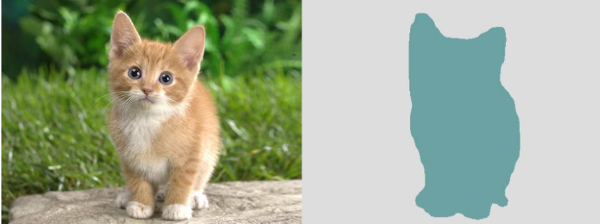
Image segmentation 分爲 semantic segmentation 和 instance segmentation, 差異如下圖：

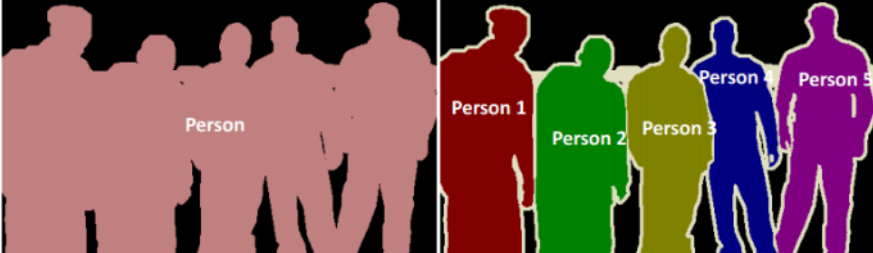
顯然 instance segmenation 比 semantic segementation 更困難。本文的 image segmentation 是 semantic segmentation.

Image Segmentation Performance Metrics (IoU, mIoU)

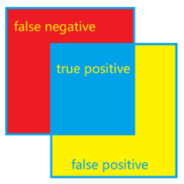
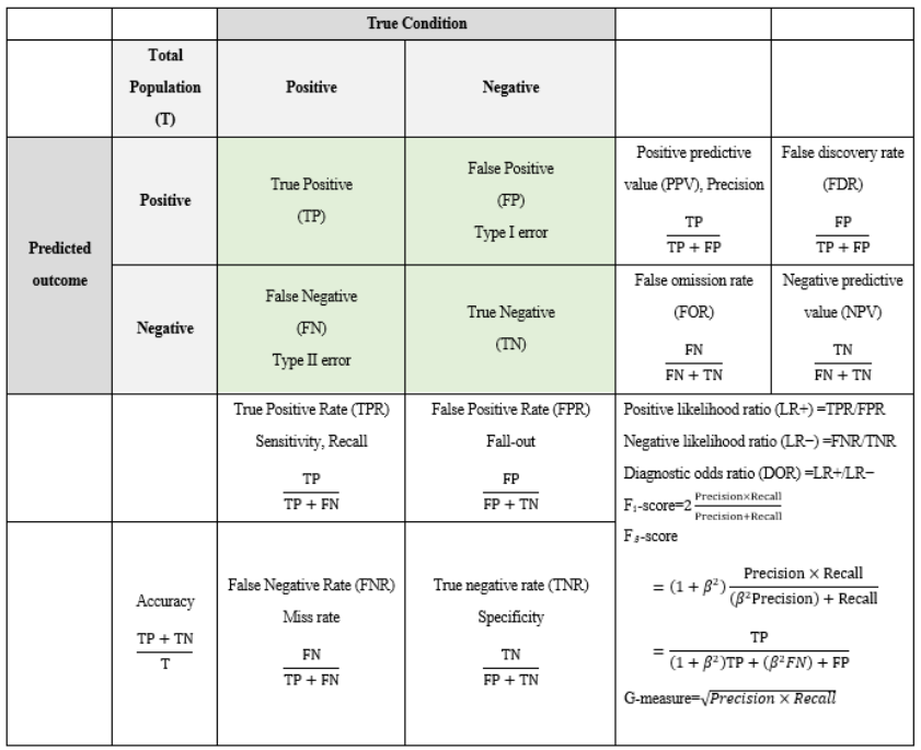
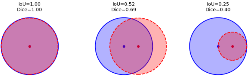
最常見的 performance metric 就是 IoU (Intersection-Over-Union) and Dice, 兩者的差異由下列公式和圖示看出： $\operatorname{IoU}(A, B)=\frac{\|A \cap B\|}{\|A \cup B\|}, \quad \operatorname{Dice}(A, B)=\frac{2\|A \cap B\|}{\|A\|+\|B\|}$

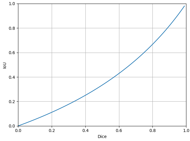
\[\text { IoU }=\frac{T P}{T P+F P+F N}, \quad \text { Dice }=\frac{2\, T P}{2\, T P+F P+F N}\] \[\text { IoU }=\frac{Dice}{2 - Dice}, \quad \text { Dice }=\frac{2 \, IoU}{1 + IoU}\]

下圖紅色的正方形是 ground truth. 藍色的正方形是 predicted outcome.

IoU (or Dice) 和一般的 precision = $\frac{TP}{TP+FP}$ and recall = $\frac{TP}{TP+FN}$的定義稍有不同。

Both IoU and Dice 介於 (含) 0 and 1. 並且 IoU $\le$ Dice. 等號只有在 IoU or Dice = 1 (和 ground truth 完全重合) 或 0 (和 ground truth 完全不沾邊) 成立。下面的例子也可以看出 IoU 和 Dice 的大小關係。一般我們用 IoU.

IoU 是針對一個 class (e.g. person) 的結果。mIoU (mean IoU) 是對所有 classes (e.g. sky, sidewalk, etc.) 的平均結果。

Loss Function

The energy function is computed by a pixel-wise soft-max over the final feature map combined with the cross-entropy loss function

UNet uses a rather novel loss weighting scheme for each pixel such that there is a higher weight at the border of segmented objects. This loss weighting scheme helped the U-Net model segment cells in biomedical images in a discontinuous fashion such that individual cells may be easily identified within the binary segmentation map.

First of all pixel-wise softmax applied on the resultant image which is followed by cross-entropy loss function. So we are classifying each pixel into one of the classes. The idea is that even in segmentation every pixel have to lie in some category and we just need to make sure that they do. So we just converted a segmentation problem into a multiclass classification one and it performed very well as compared to the traditional loss functions.

聽起來是 two-tier loss function: tier1 是 all pixel-wise softmax (using cross-entropy loss?); tier 2 是 weighting for different pixel, 特別是 boundary 的 weighting 比較重。不過我 trace code, 只有看到 cross-entropy loss?

實際的 PyTorch code [sankesaraUNet2019] 可參考 reference A

Appendix

Appendix A: PyTorch Code Review (Kaggle Segmentation of OCT Image, DME)

UNet 的結構 (forward) 包含 Encoder, Bottleneck, Decode 三個部分

Encode 非常簡單：就是 3 個 (contracting block + MaxPool2D), (比上圖的結構少一層)

Contracting block：(Conv2d+ReLU+BatchNorm) + (Conv2d+ReLU+BatchNorm)

好像不需要把 MaxPool2D 放在 contracting block 外面？

Bottleneck block 次簡單：最後一層 up-sample by 2

(Conv2d+ReLU+BatchNorm) + (Conv2d+ReLU+BatchNorm) + ConvTranspose2d : (Stride=2 for up-sampling). => 其實和 expansive block 相同，只是沒有 crop-and-concat.

Decode 比較麻煩：多了 short-cut, 也是 3 個 (cat + expansive block)

Expansive block : (Conv2d+ReLU+BatchNorm) + (Conv2d+ReLU+BatchNorm) + ConvTranspose2d : (Stride=2 for up-sampling x2)

最後一個 expansive block 稱爲 final block. 因爲不需要再 up-sampling, 把 ConvTranspose2d 改回 Conv2d+ReLU+BatchNorm

import torch
from torch import nn
import torch.nn.functional as F
import torch.optim as optim

class UNet(nn.Module):
    def contracting_block(self, in_channels, out_channels, kernel_size=3):
        block = torch.nn.Sequential(
                    torch.nn.Conv2d(kernel_size=kernel_size, in_channels=in_channels, out_channels=out_channels),
                    torch.nn.ReLU(),
                    torch.nn.BatchNorm2d(out_channels),
                    torch.nn.Conv2d(kernel_size=kernel_size, in_channels=out_channels, out_channels=out_channels),
                    torch.nn.ReLU(),
                    torch.nn.BatchNorm2d(out_channels),
                )
        return block
    
    def expansive_block(self, in_channels, mid_channel, out_channels, kernel_size=3):
            block = torch.nn.Sequential(
                    torch.nn.Conv2d(kernel_size=kernel_size, in_channels=in_channels, out_channels=mid_channel),
                    torch.nn.ReLU(),
                    torch.nn.BatchNorm2d(mid_channel),
                    torch.nn.Conv2d(kernel_size=kernel_size, in_channels=mid_channel, out_channels=mid_channel),
                    torch.nn.ReLU(),
                    torch.nn.BatchNorm2d(mid_channel),
                    torch.nn.ConvTranspose2d(in_channels=mid_channel, out_channels=out_channels, kernel_size=3, stride=2, padding=1, output_padding=1)
                    )
            return  block
    
    def final_block(self, in_channels, mid_channel, out_channels, kernel_size=3):
            block = torch.nn.Sequential(
                    torch.nn.Conv2d(kernel_size=kernel_size, in_channels=in_channels, out_channels=mid_channel),
                    torch.nn.ReLU(),
                    torch.nn.BatchNorm2d(mid_channel),
                    torch.nn.Conv2d(kernel_size=kernel_size, in_channels=mid_channel, out_channels=mid_channel),
                    torch.nn.ReLU(),
                    torch.nn.BatchNorm2d(mid_channel),
                    torch.nn.Conv2d(kernel_size=kernel_size, in_channels=mid_channel, out_channels=out_channels, padding=1),
                    torch.nn.ReLU(),
                    torch.nn.BatchNorm2d(out_channels),
                    )
            return  block
    
    def __init__(self, in_channel, out_channel):
        super(UNet, self).__init__()
        #Encode
        self.conv_encode1 = self.contracting_block(in_channels=in_channel, out_channels=64)
        self.conv_maxpool1 = torch.nn.MaxPool2d(kernel_size=2)
        self.conv_encode2 = self.contracting_block(64, 128)
        self.conv_maxpool2 = torch.nn.MaxPool2d(kernel_size=2)
        self.conv_encode3 = self.contracting_block(128, 256)
        self.conv_maxpool3 = torch.nn.MaxPool2d(kernel_size=2)
        # Bottleneck
        self.bottleneck = torch.nn.Sequential(
                            torch.nn.Conv2d(kernel_size=3, in_channels=256, out_channels=512),
                            torch.nn.ReLU(),
                            torch.nn.BatchNorm2d(512),
                            torch.nn.Conv2d(kernel_size=3, in_channels=512, out_channels=512),
                            torch.nn.ReLU(),
                            torch.nn.BatchNorm2d(512),
                            torch.nn.ConvTranspose2d(in_channels=512, out_channels=256, kernel_size=3, stride=2, padding=1, output_padding=1)
                            )
        # Decode
        self.conv_decode3 = self.expansive_block(512, 256, 128)
        self.conv_decode2 = self.expansive_block(256, 128, 64)
        self.final_layer = self.final_block(128, 64, out_channel)
        
    def crop_and_concat(self, upsampled, bypass, crop=False):
        if crop:
            c = (bypass.size()[2] - upsampled.size()[2]) // 2
            bypass = F.pad(bypass, (-c, -c, -c, -c))
        return torch.cat((upsampled, bypass), 1)
    
    def forward(self, x):
        # Encode
        encode_block1 = self.conv_encode1(x)
        encode_pool1 = self.conv_maxpool1(encode_block1)
        encode_block2 = self.conv_encode2(encode_pool1)
        encode_pool2 = self.conv_maxpool2(encode_block2)
        encode_block3 = self.conv_encode3(encode_pool2)
        encode_pool3 = self.conv_maxpool3(encode_block3)
        # Bottleneck
        bottleneck1 = self.bottleneck(encode_pool3)
        # Decode
        decode_block3 = self.crop_and_concat(bottleneck1, encode_block3, crop=True)
        cat_layer2 = self.conv_decode3(decode_block3)
        decode_block2 = self.crop_and_concat(cat_layer2, encode_block2, crop=True)
        cat_layer1 = self.conv_decode2(decode_block2)
        decode_block1 = self.crop_and_concat(cat_layer1, encode_block1, crop=True)
        final_layer = self.final_layer(decode_block1)
        return  final_layer

其他部分就是 loss (cross-entropy) 和 optimizer (SGD)

unet = Unet(in_channel=1,out_channel=2)

# Out_channel represents number of segments desired
criterion = torch.nn.CrossEntropyLoss()
optimizer = torch.optim.SGD(unet.parameters(), lr = 0.01, momentum=0.99)
optimizer.zero_grad()       
outputs = unet(inputs)

# Permute such that number of desired segments would be on 4th dimension
outputs = outputs.permute(0, 2, 3, 1)
m = outputs.shape[0]

# Resizing the outputs and label to caculate pixel wise softmax loss
outputs = outputs.resize(m*width_out*height_out, 2)
labels = labels.resize(m*width_out*height_out)
loss = criterion(outputs, labels)
loss.backward()
optimizer.step()

Use the example to compare U-Net vs. Auto-encoder by removing the short-cut!

Autoencoder 用於 image processing 第一個問題是如何 training.

dataset (label?)
loss function
supervise or self-supervised

SR,

HDR

NR,

再來我們看比較複雜的影像處理 HDR (High Dynamic Range), 代表的網路是 HDRNet