Key Message
- AI 算法的 neural network weights 是由 data training 得出,所以完全是 data dependent and determined. CV 算法多半是 fixed formula (e.g. bilinear, bicubic) 和 data 無關;最多有 parameter 可以在 post processing 人爲決定 (e.g. Lanczos-2 or Lanczos-3).
- CV resize (discrete $\to$ discrete) = interpolation (discrete $\to$ continuous) + re-sampling (continuous $\to$ discrete). 這種從 finite dimension $\to$ infinite dimension $\to$ finite dimension 是 machine learning 常見的手法,e.g. kernel SVM, deep learning 其實也算是。
我最欣賞兩種方法:
- Less is more: 大多發生在在實體設計。例如 analog design: 爲了得到 state-of-the-art performance (speed, power), 使用少數 transistors 同時做 self-bias, amplifier, offset cancellation. 另一個有名的例子是 Apple 的減法設計: one button for everything (mouse, phone, watch).
- Infinity (more) is simplicity: 大多發生在算法,所以才可能 infinity or more. 微積分是一個例子。很多 ML/DL 算法,或是本文 CV image resize 都屬於這類。
CV Image Resize
影像的放大的縮小是 computer vision 最常遇到的運算。除了因應不同的顯示尺寸 (VGA/FHD/FHD+/ 2K/2K+/4K/8K, etc.),不同的 sensor size,還要因應各種 video streaming and video call 軟體的格式。
影像的放大和縮小分別有不同的問題要解決。
Image Size Up
傳統的影像的放大或縮小是基於 interpolation (內插) 算法,通常這些內插有 analytic formula,稱為 CV 算法。
CV image size up 最大的問題是用既有資訊做內插,而且這種內插的 analytic formula 和 input data 無關。因此 ouput 無法產生新資訊 (e.g. sharper edge, details),CV 放大後的影像相對比較模糊。不同 CV 算法的差異只是相對不同程度的模糊。
這個問題一直到 deep learning 才有比較滿意的解法。主要是基於 big data 加上 overfit weight parameter 做 training/learning. 這會讓放大的影像更清晰,甚至產生細節。我們一般稱為 pixel-level AI super resolution.
AI size-up 和 CV size-up 是很好的互補。如果 input image 的 quality 還不錯 (e.g. 720p or 1080p) 以及放大的倍率不大 (e.g. < 2X),可以直接用 CV size-up 節省 computation complexity. 如果 input image 的 quality 較差,或是放大倍率大 (e.g. > 3X), 可以先用 AI 放大一個固定的倍率,在用 CV 放大剩餘的倍率。
這是 CV image size up or size down 的一個優點。因為 CV 的 analytic formula 一般可以放大或縮小任何倍率。相形之下 AI super resolution 需要固定的 input and output image size.
Image Size Down
影像的縮小並不需要產生新資訊,而是如何 preserve 既有資訊。CV 算法應該可以處理,不一定需要利用 AI 算法。但過於簡單的做法 (e.g. decimation) 會產生 aliasing 和 missing information (thin line) 問題,仍要注意避免。
CV Resize = Interpolation + Re-sampling
CV resize (包含 size up and down) 可以分解成 interpolation + re-sampling 兩個部分。
Interpolation 的 input signal 是 discrete samples with $f_s$ sampling rate; output signal 是 continuous signal.
Re-sampling 的 input signal 是 continuous signal from interpolation, output signal 是重新用 $f_r$ sampling rate 得到的 discrete samples. $f_r > f_s$ 稱爲 up-sampling; $f_r < f_s$ 成爲 down-sampling.
我們刻意强調 interpolation 是 continuous signal, 就是要把 interpolation 的 sampling rate $f_s$ 和 re-sampling 的 re-sampling rate $f_{r}$ decouple。
在 interpolation stage 完全不需要考慮 $f_r$. 不論是 $f_r > f_s$ (up-sampling), 或是 $f_r < f_s$ (down-sampling).
同樣在 re-sampling stage 完全不需要考慮 $f_s$. $f_r$ 不需要是原始 $f_s$ 的整數倍或單分數。可以是任何倍數或分數。
注意把 resize 分爲 interpolation + re-sampling, 並且引入 continuous signal 是爲了理論分析的方便。實務上 interpolation 和 re-sampling 是用 digital signal processing 整合一起運算,不會產生中間的 continuous signal.
我們先討論 interpolation, 並且引入 interpolation kernel 和 time-frequency domain analysis 得到更多 insight. 再討論 re-sampling operation.
Interpolation (Discrete $\to$ Continuous)
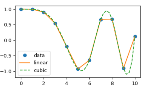
Interpolation 的觀念很直接,就是 given discrete samples (下圖綠點) 可以内插出一個 continuous signal, 稱爲 reconstructed signal. 不同的 interpolation 方式就會得到不同的 reconstructed signal. 如下圖的 linear interpolation 和 cubic interpolation 的 reconstructed signal 都是從同樣的 discrete samples 内插而來。
Interpolation Kernel
此處引入 interpolation kernel. 這是非常重要的觀念,可以抽離原始 samples 便於分析。 Reconstructed signal 就是 data sample 和 interpolation kernel 的 convolution.
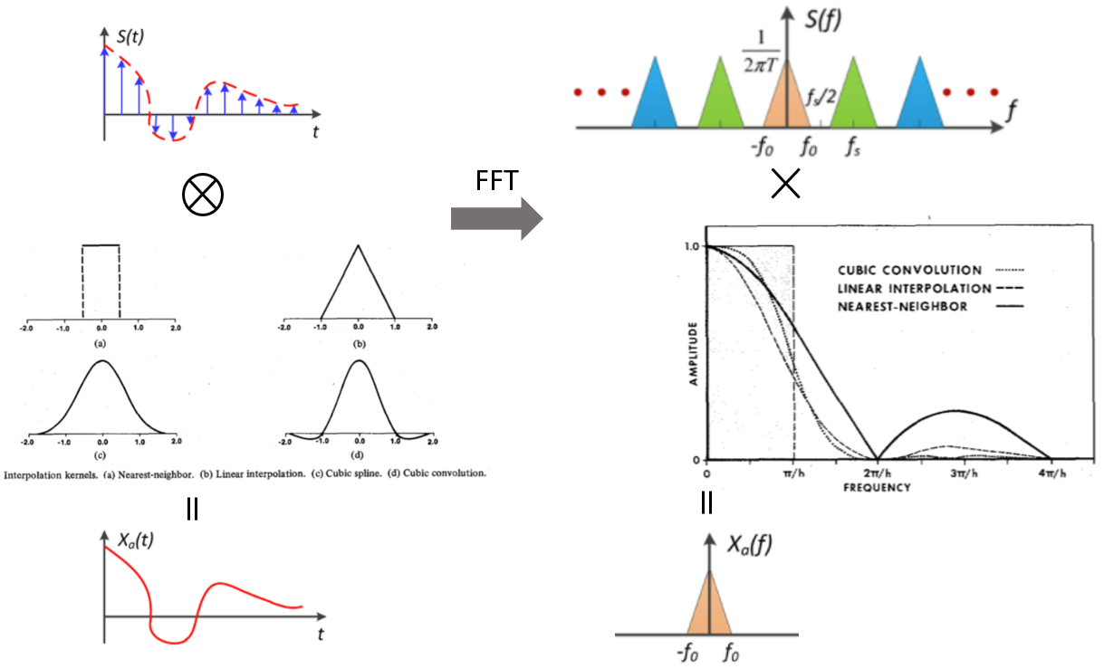
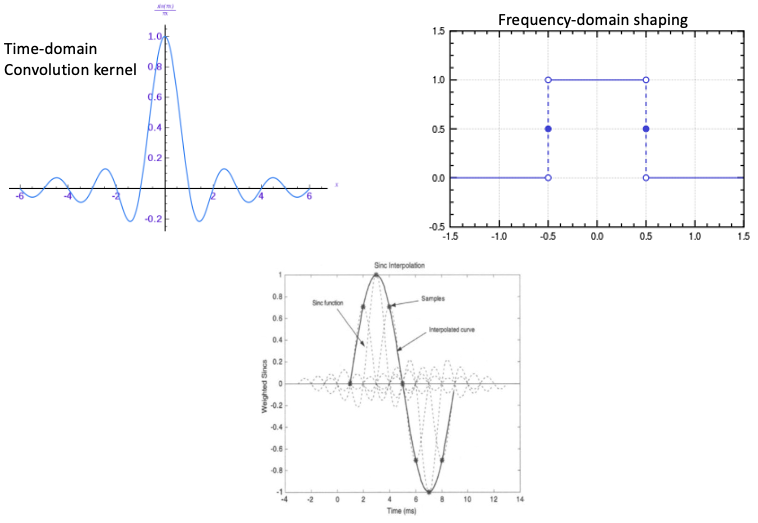
下圖左邊是 interpolation 的 time (or 2D space) domain operation, 右邊則是 interpolation 對應的 frequency domain operation. 因爲 time domain 和 frequency domain 是 conjugate, 左邊如果是 convolution, 右邊就是 multiplication; 反之亦然。
Interpolation: time domain insight
最 trivial 的 kernel 是 rectangular, 左下圖 (a). 對應的是 nearest neighbor interpolation, 得到的 reconstructed signal 就是階梯信號。
比較有意義的是 triangular kernel, 左下圖 (b), extend 到 +/-1 sample. 和 data sample 做 convolution 就會得到 linear interpolation, 如上圖橘色實綫。
比較常用的是 cubic kernel, 左下圖 (d), extend 到 +/-2 sample. Convolution 後得到 cubic interpolation, 如上圖綠色虛綫。
再來我們用 frequency domain analysis.
Interpolation: frequency domain insight
Time domain convolution 對應 frequency domain multiplication, 也就是下圖右邊的 $S(f) \times \text{FFT(kernel)}$.
理想的狀況是 FFT(kernel) 是一個 perfect low pass filter, 如右下圖的虛綫方框, i.e.
\[|\text{FFT(kernel)}| = 1 \quad \text{for} \quad f < f_s/2 \text{ (or } \pi/h)\] \[|\text{FFT(kernel)}| = 0 \quad \text{for} \quad f > f_s/2 \text{ (or } \pi/h)\]這樣可以 (1) 不影響 in-band high frequency component; (2) 移除所有 out-of-band high frequency islands centered at $ \pm f_s, \pm 2 f_s, \pm 3f_s, …$. 得到乾净的 reconstructed baseband frequency island, 如最右下圖。
Interpolation Kernel 分類
我們可以用以下的分類 interpolation kernel.
- Time (or 2D space) limited interpolation
- Frequency limited interpolation: not practical
- Frequency-shaping + time-window interpolation
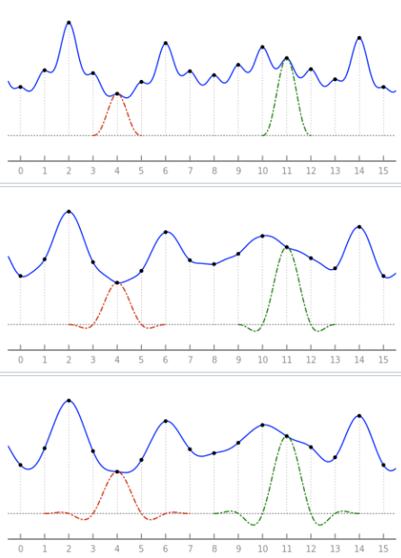
Time (or 2D Space) limited Interpolation
這類內插法非常簡單直觀,下圖顯示 1D (time) 和 2D (space) 最常見的 time/space limited 內插。灰色綫是內插的 function. 什麼是 time/space limited? 就是只用 (附近 2-4 個 for 1D, 4-16 for 2D) 有限點做內插,而不是用很多點或無限點做內插。從 convolution with interpolation kernel 的角度也很清楚,如上圖的 (a)-(d). Linear interpolation kernel 是 $\pm 1$, cubic interpolation kernel 是 $\pm 2$, 都是 time limited interpolation.
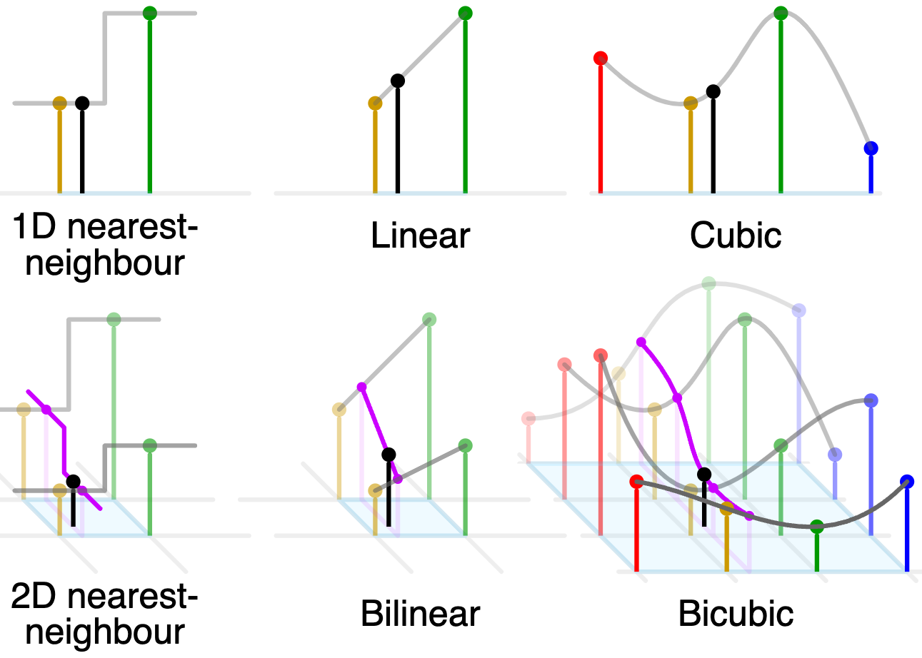
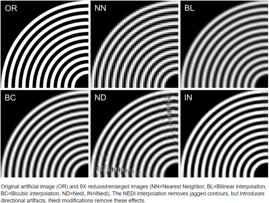
最簡單 interpolation 是 nearest neighbor, 最大的問題是誤差很大而且 boundary 非常明顯有鋸齒邊 (frequency aliasing),如下圖左。基本沒什麼人使用。從 frequency domain 分析原因是 $\text{FFT(rectangular kernel)} = sinc(f)$, 而 $sinc(f)$ 對 out-of-band high frequency islands 的抑制能力很差,如上上圖右的 nearest neighbor 實綫。
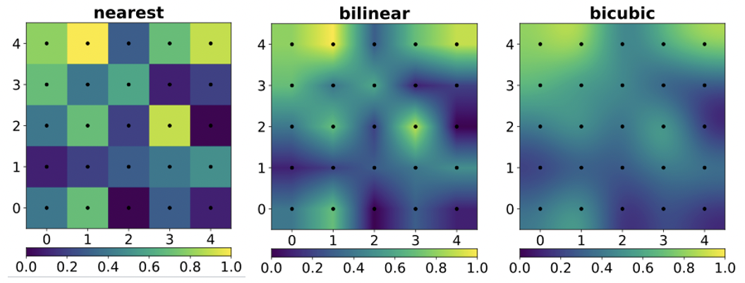
其次是 linear interpolation: 2D image 稱為 bilinear, 用四點做內插。這是常用的 interpolation, 或是作為 baseline. 主要的問題是誤差仍大會比較模糊沒有細節,如下圖中。$\text{FFT(triangular kernel)} = sinc^2(f)$, 而 $sinc^2(f)$ 對 out-of-band high frequency islands 的抑制能力比較好,如上上圖右的 linear interpolation 虛綫。
最常見的是 cubic: 用四點內插;2D 是 bicubic, 用 16 點內插。如下圖右算是比較可以接受的結果。$\text{FFT(triangular kernel)}$ 不確定是否有 close form. 實際的 frequency response 如上上圖右的 cubic interpolation 灰綫。相當程度抑制 out-of-band high frequency islands, 避免鋸齒 (good) 或 high contrast edge (may not be good). 不過一個缺點是 in-band high frequency 也被相當程度的抑制。這會造成影像的模糊 (blurred image).
Time-Frequency or Space-Frequncy 測不準原理 (Uncertainty Principle)
Fourier Transform 可以推導出測不準原理, i.e. $\Delta f(x) \cdot \Delta F(f) \ge C$ ; $f(x)$ 是 time domain function (或是 2D space domain function); $F(f) = \text{FFT(}f(x))$ 是 frequency domain spectrum. $\Delta$ 代表 variance. 兩個 conjugatge domains 的 variance product 必大於某一個值,這稱為 Uncertainty Principle of Fourier Transform. 物理意義是一個 $f(x)$ 在 time (or space) domain 愈窄 (測的愈準),$F(f)$ 在 frequency domain 就愈寬 (測的愈不準),反之亦然。這是非常 universal 的定律,也是量子力學的根基。
用於 interpolation 一個更方便的推廣是:a function cannot be both time limited and frequency band limited (i.e. not only variance) at the same instance. Basically this means that a function cannot be compactly supported in both the domains simultaneously.
舉例而言,nearest neighbor interpolation 等價於和一個 rectangular kernel 做 convolution. Rectangular kernel 是 time (or 2D space) limited ($\pm 0.5$), 所以 kernel function 的 frequency spectrum 就是延伸到無限遠。實際 $\text{FFT(rectangular kernel)} = sinc(f)$ in frequency domain. $sinc(f)$ 對於out-of-band high frequency islands 的抑制能力很差,正如 uncertainty principle 所預期。
因此 nearest neighbor interpolation 的鋸齒就代表很多的 out-of-band high frequency islands.
Linear/bilinear interpolation 是和 triangular kernel 做 convolution. Triangular kernel 雖然同樣是 time domain band limited ($\pm 1$), 但是 variance 比較大,因此對應的 $\text{FFT(triangular kernel)} = sinc^2(f)$ 雖然也會延伸到無限遠,但是高頻下降比較快 (i.e. variance 比較小), 對於 out-of-band high frequency islands 的抑制比 rectangular kernel 好。
Cubic/bicubic 同樣是 time/space domain band limited ($\pm 2$). 不過 time domain variance 更大,所以 kernel frequency spectrum 高頻下降更快,所以效果比 linear/bilinear 好!
這類 time limited interpolation kernel 雖然可以藉著 widen kernel time span 讓 frequency span 變窄以抑制 out-of-band high frequency islands, 但是 in-band high frequency component 同樣也被壓抑,因此 interpolation 之後都會看起來比較模糊 (blurred image), 缺乏 sharpness.
Frequency Limited Interpolation
另一種完全相反的 interpolation 是 frequency limited interpolation. 這類 interpolation 的好處是 (1) 完全移除 out-of-band high frequency islands; (2) 完全不影響 in-band high frequency component. 例如用下圖右的 ideal low pass filter. 因爲是 interpolation kernel 是 frequency limited, 從 uncertainty principle 我們可以預期 interpolation kernel 的 time span 是無限遠。此時的問題是需要做無限點的內插。
例一:time domain sinc resampling
如果 time/space domain interpolation 是 $sinc$ kernel (下圖左), 對應的 frequency spectrum 是 rectangular function (下圖右)。用 sinc function 做 interpolation 的做法如下圖下。
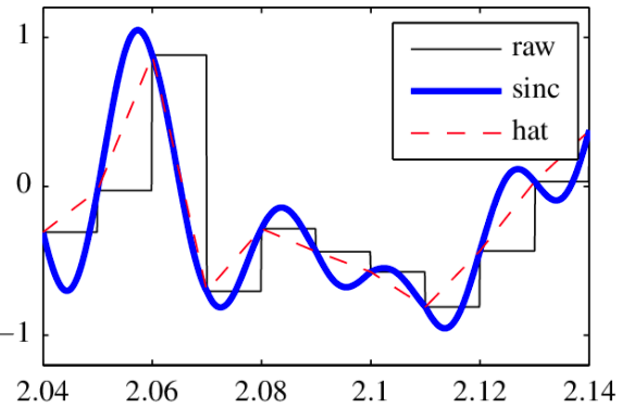
但是 $sinc$ kernel 需要無限多點做內差。這不實際,在 imagine 的應用甚至不可能。基本上所有的 image 都是有限點。不可能用 infinite time span kernel interpolation! 但 $sinc$ kernel 可以作為比較的 baseline. 下圖比較原始 (raw or nearest neighbor, 黑線), linear (hat, 紅虛線), and $sinc$ (藍線) interpolation。可以看出 $sinc$ interpolation 的效果似乎最好。
Frequency shaping + Time windowing Interpolation
這裏的想法很簡單。就是想要 trade off $sinc$ kernel interpolation to (1) 幾乎移除 out-of-band high frequency islands; (2) 幾乎不影響 in-band high frequency component, with 有限點內插。 解決的分法就是在 $sinc$ kernel 上乘一個 windowing function! 此時 kernel function 變成 time-limited. 但從 uncertainty principle 我們可以預期 kernel frequency spectrum 變成無限。所以 frequency filter從”完全移除“變成”幾乎移除“,”完全不影響“變成”幾乎不影響“。
重點是在 windowing function! 我們先 recap 頻譜分析常用的 time windowing, 暫稱爲 wide (time) scope windowing. 再回到本文的 time windowing for interpolation, 暫稱爲 narrow (time) scope windowing.
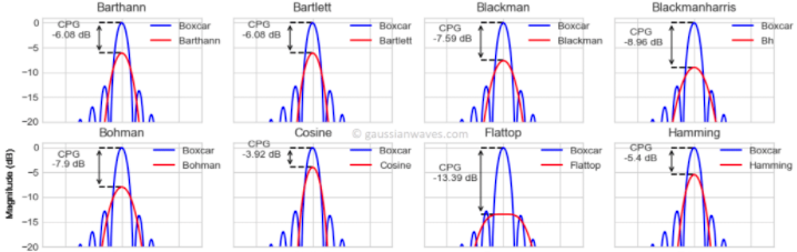
(Recap) Wide Scope Windowing for 頻譜分析
Windowing function 在 time domain 信號處理很常見,像是 hamming, hanging, kaiser windowing, etc, 如下下圖。因爲 window 是乘上 global signal, 暫稱爲 wide scope windowing.
這類 windowing 的目的是針對 narrowband signal (e.g. sine wave),需要 truncate 之後做頻譜分析失真,例如 harmonic distortion, SNR, 等等。Windowing 的做法是在 time domain waveform 乘上 windowing function, 如下圖。
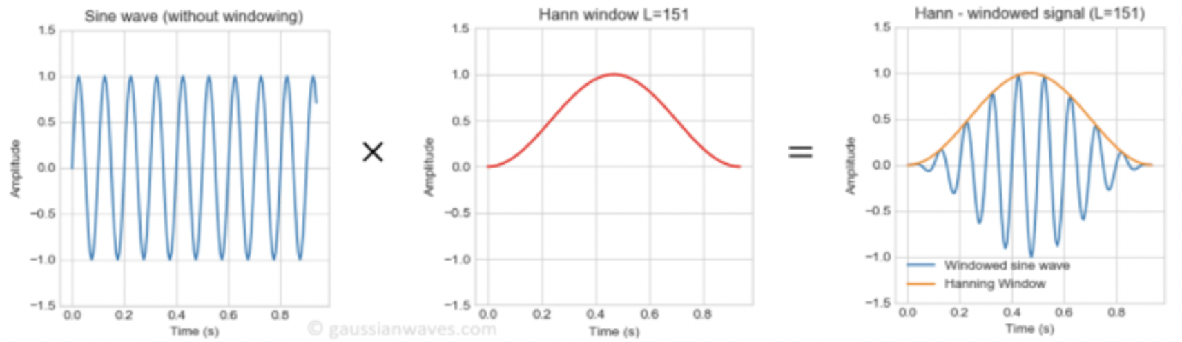
Time domain windowing multiplication 對應的是 frequency domain convolution with FFT(windowing).
直接 truncate time domain waveform 等價乘上 rectangular function, 對應是 frequency domain convolution with a $sinc$ function, 就是下圖所有的藍色 reference trace. 這裏最大的問題是 $sinc$ function 有很多 sidelobe, 和 narrowband singal convolution 後會影響 narrowband signal 對於 harmonics 和 noise 的判斷。這也稱為 frequency leakage problem.
Wide scope window function 主要的作用就是減低 sidelobe at the expense of wider mainlobe. 我最常用的 window function 是 Kaiser function with parameter = 12.4 to trade off the sidelobe suppression and mainlobe width.
(Back to) Local Scope Windowing for Interpolation
Narrow scope windowing 主要的目的 windowing interpolation kernel 避免無限點內插 and apply the windowed kernel to every sample for interpolation. 因爲 windowing function 是 apply 在每一個 sample 附近的 kernel,所以暫稱爲 local scope windowing.
我們直接看例子。
Lanczos Interpolation
http://checko.blogspot.com/2005/04/resize-bicubic-bilinear.html
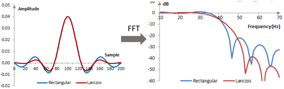
Lanczos interpolation 就是 $sinc$ interpolation funtion 再乘上 truncated sinc windowing function. 所以 Lanczos interpolation kernel 在 time/space domain 是 finite, 但在 frequency domain 變成無限。 (a 是 design parameter)
\(L(x)= \begin{cases}\operatorname{sinc}(x) \operatorname{sinc}(x / a) & \text { if }-a<x<a \\ 0 & \text { otherwise. }\end{cases}\) Equivalently, \(L(x)= \begin{cases}1 & \text { if } x=0, \\ \frac{a \sin (\pi x) \sin (\pi x / a)}{\pi^{2} x^{2}} & \text { if }-a \leq x<a \text { and } x \neq 0, \\ 0 & \text { otherwise. }\end{cases}\) 下圖左是 Lanczos (i.e. sinc kernel with sinc window) vs. sinc kernel with rectangular window at time domain. 下圖右是其對應的 frequency spectrum in log scale. 可以看到 time domain apply windowing (i.e. time-limited) 會造成 frequency spectrum 變爲無限。但是 sinc window (Lanczos) 比起 rectangular window 對於 out-of-band frequency islands 的抑制好的多 (>20dB), 但是 in-band high frequency 也略微衰減。不過比起 bi-linear interpolation 或是 bi-cubic interpolation, in-band high frequency 還是好的多! 這也是爲什麽 Lanczos interpolation 效果比起 Bicubicle 更好的原因。
Lanczos-a 的 a 是 interger parameter. 決定 time domain 的 windowing scope, 如下圖。
- a=1 的 scope 介於 $\pm 1$; a=2 的 scope 介於 $\pm 2$; a=3 的 scope 介於 $\pm 3$
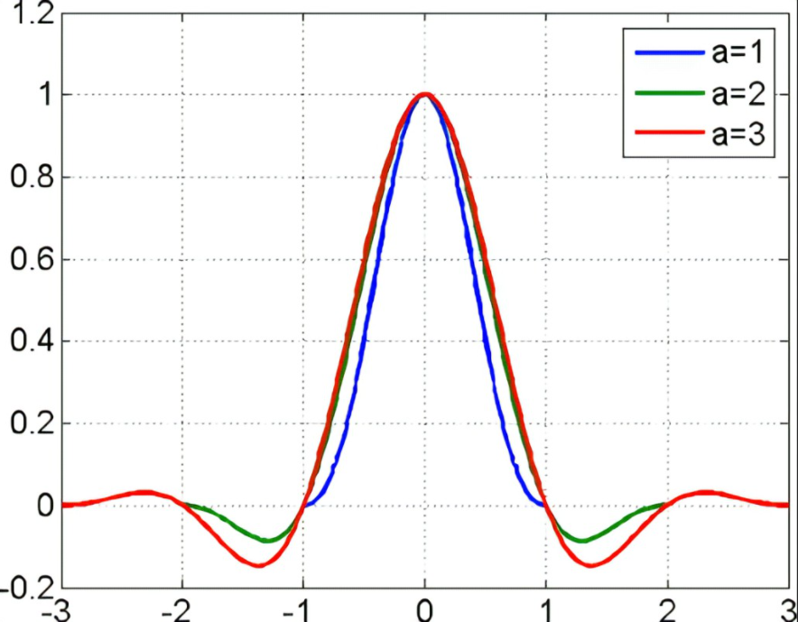
Lanczos-1/2/3 Interpolation 的結果如下圖。a=1 明顯不佳,out-of-band high frequency islands 抑制不足,實務上很少用。
a = 2 and a = 3 效果接近。一般會用 a = 2 或 a = 3 (e.g. Adobe) for interpolation.
Window 的應用和效果可以整理如下表。
| Wide scope windowing for 頻譜分析 | Local scope windowing for interpolation | |
|---|---|---|
| Input signal | Narrowband signal (with harmonic, noise, etc.) | Broadband signal (speech, image) |
| Purpose | Reduce frequency leakage during truncation | Avoid infinite samples interpolation by trading off frequency shaping |
| Window scope | Global; one window multiply the global samples | Local; many windows, each window multiply the local vicinity samples |
| Window | Hamming, Hanning, Kaiser, etc. | Lanczos (sinc kernel with sinc window) |
Interpolation Summary
總結三種不同的 interpolation 方式,可以看出最常用的是 bicubicle (shoot for lowest interpolation complexity) 或是 Lanczos (best quality with slightly higher interpolation complexity).
| Interpolation type | Time/space limited | Frequency limited | Frequency-shaping + time-window |
|---|---|---|---|
| Example | Bilinear, Bicubicle | Infinite sinc | Lanczos (sinc kernel with sinc window) |
| Suppress out-of-band high frequency islands | Billinear: bad; Bicubicle: good | Excellent | Good |
| Keep in-band high frequency intact | Bad | Excellent | Good |
| Interpolation complexity | Low (few samples and linear or cubic function) | Infinite and infeasible | Low-Medium (few samples but sinc funcions) |
(Re)-Sampling (Continuous $\to$ Discrete)
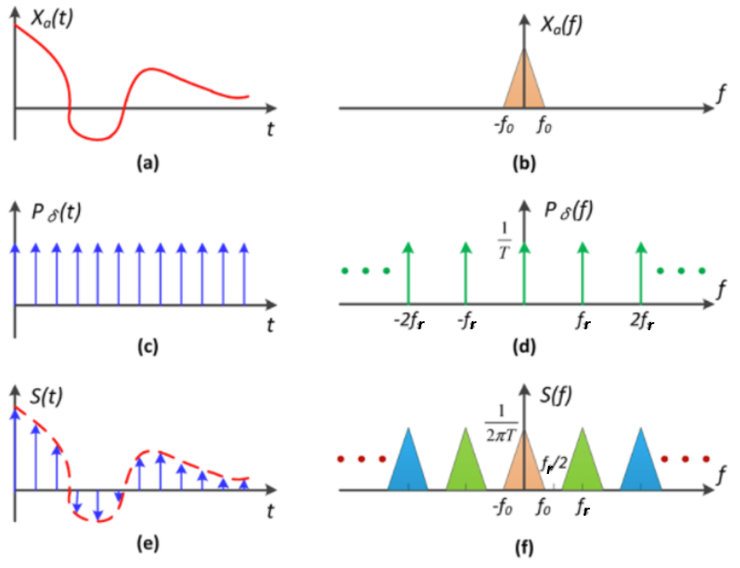
前面已經完成 interpolation 得到 reconstructed signal, $X_o(t)$, 如下圖 (a). 其對應的 frequency spectrum, $X_o(f)$, 如下圖 (b).
數學上 (re)-sampling 就是乘上 Shah function, $P_{\delta}(t)$, 如下圖 (c) and (e) [bevelShahFunction2011]. Shah function 的 frequency spectrum 也是 Shah function, $P_{\delta}(f)$, 不過兩者的間距是倒數關係。Samplling process 就是在 time domain 乘上 $P_{\delta}(t)$, frequency domain 對應的是 convolution with $P_{\delta}(f)$, 如下圖 (d) and (f) 1.
Re-sampling Issues
Re-sampling 包含 up-sampling and down-sampling. 決定於上圖 (c) 的 Shah function 的間距,就是 re-sampling frequency, $f_r$. 如果 $f_r > f_s$ 爲 up-sampling; 反之稱爲 down-sampling. 通常 re-sampling frequency $f_r$ 是 $f_s$ 的整數倍 (x2, x3, etc.) 或是單分數 (1/2, 1/3, etc.),但並不一定需要。
CV resize 的特點就是 decouple interpolation frequency and re-sampling frequency. Re-sampling 不必是原始 sample frequency 的整數或單分數,可以任意選擇 $f_r$。相反 AI resize 一般是一個固定倍數, e.g. x1.5, x2, x3, etc. 這是 CV resize vs. AI resize 的一大優點。
From digital sampling theorem 和 Fourier transform 看 up-sampling 和 down-sampling 會遇到的問題。
-
Up-sampling ratio 越大 ($f_r \gg f_s$): $P_{\delta}(t)$ 愈密,$P_{\delta}(f)$ 愈疏,兩者的間距是倒數關係。Down-sampling 剛好相反。
-
Up-sampling 把 out-of-band high frequency islands 的距離拉大,最大的問題:
- 等效是 in-band high frequency information void. 高頻無法無中生有,影像缺乏高頻細節,感覺變模糊 (blurred).
- 如果原來的 in-band high frequency component 就很大,距離拉開可能會造成 in-band high frequency 和 out-of-band overlapping frequency (i.e. frequency aliasing) 的改變,也有可能造成問題, e.g. down convert some high frequency pattern to low frequency 像是摩爾紋 (?)。
-
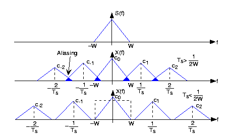
Down-sampling 把 out-of-band frequency islands 的距離拉近,最大的問題:
- High frequency aliasing 如下圖藍色重叠部分。影像多出 spurious frequency, i.e. 出現亮度或顏色突然變化的雜點,或是消失的細節或斷線。
- 爲了減少 high frequency aliasing, 經常會先用 prefiltering apply to orignal signal. 這又會造成 in-band high frequency attenuation, 影像變模糊。
下表整理上述重點:
| Issue | Up-sampling | Down-Sampling |
|---|---|---|
| Frequency aliasing | 鋸齒或補丁 pattern, 摩爾紋。 | 多出 spurious frequency, i.e. 出現亮度或顏色突然變化的雜點,或是消失的細節或斷線。 |
| Frequency shaping | NA | down-sampling 高頻消失變 aliasing, 比較好的算法會使用 prefiltering to avoid aliasing, 整體影像變模糊 |
| Frequeny missing | 高頻無法無中生有,影像變模糊 (blurred). | NA |
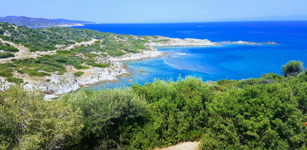
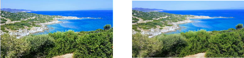
Down-Sampling Example
下圖上是大圖。經過簡單縮圖 using Bitmap’s CreateScaledBitmap() 的結果如下圖左下。因為 frequency aliasing 的圖有比較多的 spurious 高頻成分,看起來好像比較多細節, 但是失真多,例如海面上很多雜點。使用 prefiltering to avoid aliasing 的結果如下圖右下。Prefiltering 避免 aliasing, 但是因為縮圖 down sampling 本身會損失高頻解析度,所以一些細節如樹叢,沙灘會變模糊。一般我們還是 prefer 下圖右,雖然視覺上可能覺得下圖左比較豐富。這也許是 AI 算法可以幫忙的地方,例如先分區,再 apply 不同的 CV algorithm.
再來我們非常 high level 比較 CV image resize vs. AI image resize (usually size up, i.e. super resolution) vs. mixed AI&CV resize.
CV Image Resize Vs. AI Image Resize
下表 summarize pixel level AI image size up vs. CV image size up/down. 也粗略討論 mixed AI and CV image resize. CV 算法一般只能處理 out-of-band frequeny islands aliasing 和 in-band high frequency shaping issues, 且兩者常常是 trade-off.
CV 算法一般是 content independent. 所以不大可能無中生有,因此 CV 算法無法處理 high frequency void from up-sampling.
Pixel-level AI super resolution (AISR) 是 content dependent, 可以 training to keep in-band high frequency content for sharper edge and better constrast. 甚至可以生成 missing frequency component. 當然 pixel-level AISR 的缺點是計算資源太大,同時大多只能放大固定倍率。
| AI size up (SR) | CV size up | CV size down | Mixed AI & CV resize (E.g. AI for zoning; CV for pixel processing) | |
|---|---|---|---|---|
| Pro | Good image quality: sharp edge, more details | Low computing complexity, typical with analytical form; flexible input or output image size | Low computing complexity, typical with analytical form; flexible input or output image size | Computation complexity between pixel-level AI and CV; and the quality is also in-between |
| Con | Fixed input/output image size; high computing complexity | Blurred image quality; artifact from aliasing | Trade-off between sharpness (prefilter remove high frequency) and aliasing (spurious high frequency) | The opposite of Pro. Computation > CV; Quality < AI. |
| Issue | Need big data for learning | Unable to generate missing details | NA | Unable to generate missing details |
Continuous interpolation scaling (CV) vs. Pyramid scaling (NN )
AI + NN
Cascade, Parallel, Fuse?
Reference
-
完整的 sampling process, 會在下圖 (e) step 之後,再 convolve with a narrow rectangular function, 變成階梯 function. 這更接近在顯示器的狀態。此處忽略。 ↩