Math AI Flow and Flux PDE

”流 (Flow)“ 或 “波 (Wave)” 的偏微分方程 (PDE)

“流 (flow)” 或是 “波 (wave)” 都是常見或常感知的現象，例如水流、水波、寒流、熱流。 Flow or wave 是時間和空間連續或整體行爲 (global or continuous behavior over space and time). 我們不會只看水中單點瞬間的運動判斷這是一個 flow or wave, 因爲可能是水流，水波，甚至渦流。因此需要分析時間和空間連續或整體行爲。如何進行?

有幾種方式：

1. 利用連續性 (bottom-up approach): 用偏微分方程描述每一點附近空間和時間的關係。藉著解偏微分方程 (PDE)，可以得到整體的行爲。一般的 CV (computer vision) approach, 基本都和 PDF 的解法有關。
2. 把 PDE 轉換成積分形式，例如 Maxwell PDE equation 的積分形式。此時已經不是只描述局部行為，而是一個區域或是整體的行為。一般積分形式是為了闡述物理意義，直接求解很困難。但如果可以把解 PDE 轉換成 (積分) cost function optimization，就可以：(1) 利用 deep neural network 近似這個 cost function; (2) 使用 real data training for optimization 得到近似解。
3. 直接描述整體行爲 (up approach)：例如電路學用 KVL, KCL (Kirchikov Voltage/Current Laws) 簡化代替 Maxwell equations，並且定義電阻、電容、電感等，取代 local transport equation. 或者用熱力學代替統計力學，電子學代替固態物理學。雖然只能得到簡化的 high level solution. 不過在很多實際應用，這樣 high level solution 已經足夠，例如電子電路分析，或是 IC 散熱分析。

本文 focus on PDE 因爲可以看到更基本的物理意義。如上所述，要描述每一點附近空間和時間的關係，需要定義

**(1) 每一點 (空間和時間)要描述的物理量, e.g. (scalar) density, driving force, (vector) flux/motion; **

**(2) 物理量和時間的關係, continuity equation; **

**(3) 物理量對空間的關係, transport equation; **

(4) combine continuity equation and transport equation 得到完整的 flow or wave PDE.

每一點 (空間和時間) 物理量：flux (通量)

Flux 是一個向量 (或是向量場)，描述 magnitute and direction of the flow for transport phenomen. 簡單說就是帶有方向的 flow rate per unit area. 此處的 flow 可以是物質 (substance) 例如 water, particles; 或是特性 (property) 例如 heat, light, energy, E-field/M-field/EM-field, or motion (?). 很多時候 flux 的方向是物質移動的方向，例如水流，但不是絕對。例如在水波或是橫波，物質移動的方向和 energy flux 就不一致。

• Magnitute

• Direction

另外一個 flux 定義是 flux vector 對一個 surface 的積分，e.g. 磁通量，電通量。這是整體的行爲，其實可以稱爲 flow.

Flux 和時間的關係，一般由 continutity equation 決定, e.g. $\nabla \cdot \mathbf{J} + \frac{\partial \phi}{\partial t} = 0$

Flux 和空間的關係，一般由 transport equation 決定, e.g. $\mathbf{J} = - \nabla V$

如何產生 flow (0th order and 1st order in time)?

Simple: 要有 driving force; i.e. potential.

Simple Transport: to follow the driving force.

如果 flux diverge 對時間的積分為 0 或又和 potential 成正比，就會形成 flow.

如何產生 wave (2nd order in time)?

1. transport equation 的 substance local motion 和 driving force (potential) 行進方向垂直，因此可以 back-and-force (位能-動能 or 電能-磁能)! 產生 wave! (橫波)
2. lag in time, 所以產生 back-and-force wave (縱波)
3. transport equation 本身就含有 time dependence (水波)

Continuity Equation of Flux

• 如果是 incompressible flow, flux 的散度 $\nabla \cdot \mathbf{J} = 0$, 這是很強的條件，一般只有在 (1) incompressible substance, 例如水或液體 flow; (2) static or stationary flux vector field, 才會成立; (3) From Maxwell equation, both stationary or time-varying 的電場 (no charge location) 和磁場都可以視爲是 incompressible flow! ($\nabla \cdot \mathbf{E} = 0; \nabla \cdot \mathbf{B} = 0$). Incompressible flow 的物理意義很單純，就是進入一個 volumn 的 flow 等於出去的 flow, 不會有局部的 mass, energy, momentum, charge 的累積。

• 比較 general 的 flow 會滿足 continuity equation, 如下式。 $\phi$ 可以是 mass, energy, momentum, charge 等可以守恆量。

\[\nabla \cdot \mathbf{J} + \frac{\partial \phi}{\partial t} = 0 \label{cont}\]

• 下一步我們想瞭解的是 flux 的旋度, $\nabla \times \mathbf{J}$, 旋度的物理意義也很直觀，就是判斷 flow 是否帶有漩渦，渦流，層流。旋度為 0 的 flow, $\nabla \times \mathbf{J} = 0$, 稱為 irrotational flow 無旋流 (i.e. 平直流)，如下圖。具有重要的意義，就是任兩點的路徑積分都相同。或是路徑積分只和起點和終點有關，和路徑無關。數學上可以定義一個 ”勢“函數 (potential function)，使得 $-\nabla V = \mathbf{J}$. 也是由於這個勢能差，才會造成 flow.
  • 很多簡單物理流滿足 irrotational flow, 例如 heat flow 由於溫度差；diffusion flow 由於濃度差。直覺上 heat flow or diffusion flow 不會旋轉，應該屬於平直流。事實也是如此。
  • 還有 static and quasi-static 電場 (或磁場) ，$\nabla \times \mathbf{E} \approx 0$, $-\nabla V = \mathbf{E}$, 對應的勢能 (場) 就是電壓 (場)。
  • 但很多比較複雜的 flow 都不是 irrotational flow，如水湍流，氣流，電磁場，甚至 property flow 如光流，都可能有局部或是 global 旋流/渦流。本文暫不討論。
• 注意此處的 $V$ ，不同於上式的 $\phi$. $V$ 是 $\mathbf{J}$ 對空間的線積分；$\phi$ 則是 $\nabla\cdot \mathbf{J}$ 對於時間的積分。兩者的單位不同。物理意義也不同：$V$ 是勢能；勢能差造成 flux/flow. $\phi$ 是 flux 進出差 (i.e. divergence ) 纍積的物理量，就是守恆量 (mass, energy, momentum, charge)。

Transport Equation of Flux

有趣的是，$V$ 和 $\phi$ 常常都有簡單的關係，稱爲 transport equation (spatial dependent)。以下是一些 flow 例子：

Diffusion Flow

Continuity equation, 也代表質量守恆 equation. \(\nabla \cdot \mathbf{J} + \frac{\partial \varphi}{\partial t} = 0 \label{DiffCont}\) where

• $\mathbf{J}$ is the diffusion flux, measures the amount of substance that will flow through a unit area during a unit time interval.

• φ (for ideal mixtures) is the concentration, of which the dimension is amount of substance (mole) per unit volume.

再來因爲 diffusion flux 是 irrotational flow, $\nabla \times \mathbf{J} = 0$, 而且 potential $V$, $-\nabla V = \mathbf{J}$. 也就是驅動 diffusion flux 的勢能 $V$. 在 diffusion flux 的例子，$V$ 剛好正比于 $\varphi$, 也就是 $ V = D \varphi \rightarrow \mathbf{J} = -\nabla V = -D \nabla \varphi$. 這個比例常數, $D$, 稱爲 diffusion constant.

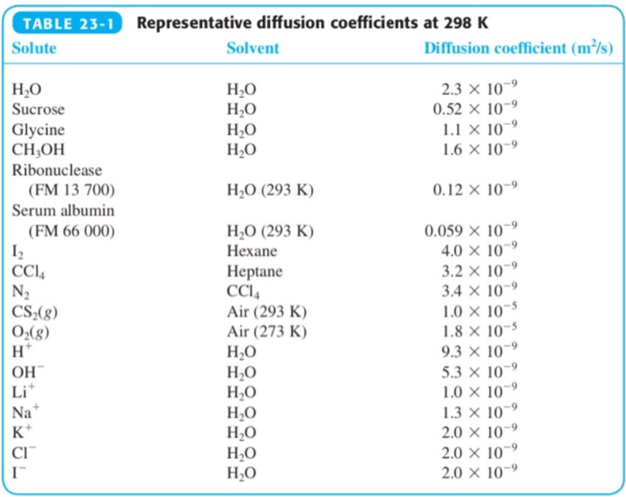
這就是 Fick’s first law, 也稱爲 transport law. \(\mathbf{J} = - D \nabla \varphi \label{Fick1}\) 爲什麽不是用 $V$ 取代 $\varphi$, 把比例常數放在另一邊，such as $\varphi = D’ V \to D’ \mathbf{J} = -\nabla V$? 主要的原因是 continuity equation including $\mathbf{J}$ and $\varphi$ 更基本，而 $V$ and $D = V / \varphi$ 則 depends on material and environment (e.g. 溫度，溶劑)，如下表。

$D$ 除了反應 material 和 environment 的特性，另一個功能吸收收 $V$ and $\varphi$ 單位的差異, area per unit time $L^2/T$, or SI 單位 $m^2/s$. 對於類似的 transport phenomen都是同樣的單位，

結合 continuity equation 和 transport law，就得到有名的 Fick’s second law (or transport equation) PDE (partial differential equation) with Laplacian operator. 在 Steady state 就化簡成 Laplacian equation. \(\frac{\partial \varphi}{\partial t} = D \nabla ^ 2 \varphi = D \Delta \varphi \label{Fick2}\)

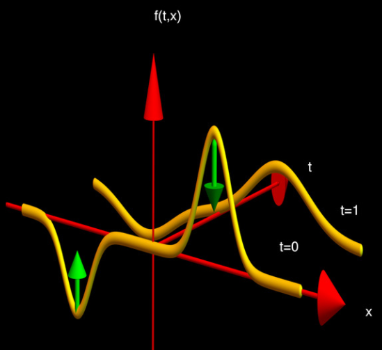
我們可以推論一下 $\varphi$ 的定性分析。我們簡化 $\nabla^2 \varphi = \Delta \varphi$ 為 1D spatial domain, 物理意義就是曲率。

• 對於凸函數曲率為負值，因爲 $D$ 是正值，所以代表 $\varphi$ 對時間的微分為負值。因此凸函數隨時間變平緩，如下圖右半。
• 對於凹函數曲率為正值，因爲 $D$ 是正值，所以代表 $\varphi$ 對時間的微分為正值。因此凹函數隨時間變平緩，如下圖左半。
• 因此隨時間增加，山峰會平緩，山谷也會變平坦。這和熱或擴散的物理直覺一致，會到達熱平衡或濃度平衡。

$\eqref{Fick2}$和 heat equation $\eqref{HeatEq}$ 其實一模一樣。只是把 diffusion constant $D$ 改成 thermal conductivity $k$。上式 fundmantal solution 稱爲 (heat) kernel. 基本是 variance 隨時間變大的 Gaussian function. 當然 PDE 具體問題的解 depends on the boundary condition.
\(\varphi(x, t)=\frac{1}{\sqrt{4 \pi D t}} \exp \left(-\frac{x^{2}}{4 D t}\right) \label{HeatKern}\)

最後一步，如何求解 flux vector field? 只要把 scalar field $\varphi$ 取 gradient in $\eqref{Fick1}$ 就可以得到 flux vector field $\mathbf{J}$.

Heat Flow

熱大概是和日常生活經驗最相關，但又比較多樣性的物理量。這不是單指今天的溫度 (C/F/K)冷熱；還有（食物）熱量 (J/Cal/Kcal)；熱力學的熱容 (量) ($J/K$)；各種物體的比熱 ($J/(Kg\cdot K)$)；電腦的散熱片的熱阻 (K/W or C/W) 或熱導 (W/K). Wiki 做了一個 thermal 和 electrical 的類比如下，可以更容易理解。[wiki 熱阻]

type	Diffusion	Incompress Fluid	Thermal	Electrical	structural
Conserved quantity	Substance 濃度 $\varphi\,[mol/m^3]$	volume $V\,[m^3]$	熱量 $Q\,[J]$	電荷 $q\,[C]$	impulse $J\, [N·s]$
potential	濃度梯度 $\nabla\varphi\,[mol/m^4]$	壓力 $P \,[N/m^2]$	溫度 $T\, [K]$	電壓 $V\,[V = J/C]$	displacement $X\, [m]$
flow rate	diffusion rate $[mol/s]$	flow rate $Q \,[m^3/s]$	heat transfer rate $\dot{Q}\,[W = J/s]$	電流 $I\,[A = C/s]$	load or force $F\, [N]$
flux (density)	diffusion flux density $\mathbf{J}\, [ mol/(m^2·s)]$	velocity $\mathbf {v}\, [m/s]$	heat energy flux $\mathbf{q}\, [W/m^2]$	電流密度 $\mathbf {j}\,[C/(m^2\cdot s) = A/m^2]$	stress $\sigma \, [Pa = N/m^2]$
resistance	flexibility (rheology defined) [1/Pa]	fluid resistance R […]	thermal resistance $R\, [K/W]$	electrical resistance $R\, [\Omega]$	flexibility (rheology defined) [1/Pa]
conductance	… … [Pa]	fluid conductance G […]	thermal conductance $G\, [W/K]$	electrical conductance $G\,[S]$	… … [Pa]
resistivity	diffusion resistivity	fluid resistivity	thermal resistivity $[(m·K)/W]$	electrical resistivity $\rho\, [\Omega·m]$	flexibility 1/k [m/N]
conductivity	diffuse constant $D\,[m^2/s]$	fluid conductivity	thermal conductivity $k\, [W/(m·K)]$	electrical conductivity $\sigma [S/m]$	stiffness k [N/m]
lumped element linear model	Fick’s 1st law$ \Delta X=F/k$	Hagen–Poiseuille equation $\Delta P=QR$	Newton’s law of cooling $\Delta T={\dot {Q}}R$	Ohm’s law $\Delta V=IR$	Hooke’s law $ \Delta X=F/k$
distributed linear model	Fick’s 1st law $\mathbf{J} = -D \nabla \phi$		Fourier’s law $\mathbf{q} = -k \nabla T$	Ohm’s law $\mathbf{j} = \sigma\mathbf{E} = -\sigma \nabla V$

Thermal continuity equation: 也代表能量守恆 \(\nabla \cdot \mathbf{q} + \frac{\partial u}{\partial t} = 0 \label{ContHeat}\) where

• $\mathbf{q}$ is the heat energy flux, measures the amount of energy that will flow through a unit area during a unit time interval ($W/m^2$).

• $u$ local energy density, of which the dimension is energy per unit volume ($J/m^3$). 這樣上式的單位就 match.

另外需要 heat transport equation, 此處是 Fourier’s law. 這個比例常數, $k$, 稱爲 thermal conductivity, [$W/(K·m)$] \(\mathbf{q} = -k \nabla T \label{fourier}\)

這裏和 diffusion 有一點不同是使用溫度 $T$ (and its gradient), 而不是 local energy density $u$， 因爲溫度比 energy density 更普遍，同時物體達成熱平衡時溫度趨於一致。兩者直接相關 [hancock1DHeat2006] \(u= (N/V) c_{v} k_{\mathrm{B}} T = \rho \,c\, T \label{heatcapa}\)

where

• $c_v$ 是 dimensionless specfic heat capacity (相對比熱)，對於氣體大約是 1.5-3, depending on 材料。
• $k_B$ 是波茲曼常數 ($J/K$).
• $N/V [1/m^3]$ 是單位體積的 (氣體) 粒子的數目，depending on 材料。
• 對於相同的材料，$u$ 正比於 $T$, 單位是 $J/m^3$
• $\rho$ 是密度 [$Kg/m^3$]
• $c$ 是 specific heat capacity 比熱 (容) [$J/(Kg·K)$].

結合 $\eqref{ContHeat}$, $\eqref{fourier}$, and $\eqref{heatcapa}$ 可以得出有名的 heat PDE equation, 其形式和 Fick’s diffusion PDE 完全一樣。 \(\frac{\partial u}{\partial t} = \frac{k}{\rho c} \nabla ^ 2 u = \kappa \Delta u \label{HeatEq}\)

or

\[{\rho c} \frac{\partial T}{\partial t} = k \nabla ^ 2 T\label{HeatEq2}\]

where

• $\kappa = \frac{k}{\rho c}$ [$m^2/s$] 是 thermal diffusivity; 概念和單位和 diffusion constant 一致。

IC 散熱以及 Thermal Resistance

上面介紹過熱量，溫度，比熱，thermal conductivity, thermal diffusivity. 此處順便提一下 IC 散熱常用的 thermal resistance [nelsonPackageThermal2018]. 另文再詳細介紹。

IC 和散熱分成幾個節點：

• Die 對應的是 $T_j$ , junction temperature: 熱源 (heat generator), 就是下圖淺藍色的 die 和紅色的 $T_j$.
• Package 對應的是 $T_c$ , IC top case temperature: 就是下圖灰色部分。這是散熱 path 1, 從 package 再散熱到 ambient (air) $T_a$.
• PC board 對應的是 $T_b$, PCB (surface) temperature: 就是下圖深藍色部分。這是散熱 path 2, 從 package (power/ground) balls 經 PCB traces, 最後在散熱到 ambient $T_a$.

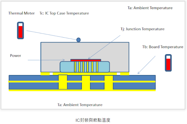
可以定義如下的 (theta) 熱阻 (thermal resistance). 並利用熱源和熱阻組成的 ”熱路” 表示散熱的路徑如下。就如同電源和電阻組成電路的概念。

\[\begin{aligned} &\Theta_{\mathrm{JA}} : \text{Junction-to-Ambient Thermal Resistance}\\ &\Theta_{\mathrm{JB}} : \text{Junction-to-Board Thermal Resistance}\\ &\Theta_{\mathrm{JC}} : \text{Junction-to-Case Thermal Resistance}\\ \end{aligned}\]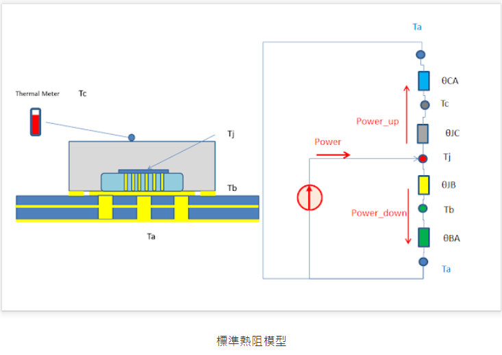

我們看一些 package 的 thermal resistance 的例子。就是 1W power 會造成溫度上升幾度。愈大就代表阻值愈大。

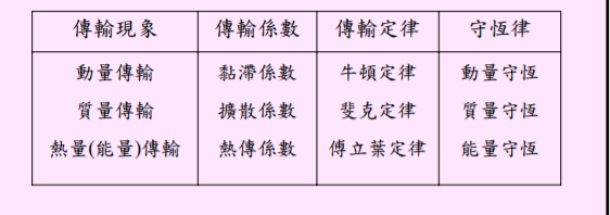
Transport Phenomenon Summary

前面討論 diffusion flux 和 heat flux. 還有類似的例如 Newton’s viscosity law 也是如此。

包含 (1) continuity equation to conserve the substance/energy/momentum; (2) transport law because of irrotatinal flux, 也就是 curl 為 0. 最後得到 diffusion equation. \(\frac{\partial \phi}{\partial t} = c \nabla^2 \phi\) 下表[Wiki] 為 summary.

Transport Phenomen	比例常數	Transport Law	Conservation
Substance flux	Diffusion constant	Fick’s diffusion law	Substance
Heat (energy) flux	Thermal conductivity/ Thermal diffusivity	Fourier’s conduction law	Energy
Momentum flux	Viscosity/Momentum diffusivity	Newton’s viscosity law	Momentum

Fluid Flow

參考 Wiki [@NavierStokes2022].

Continuity equation: concervation of mass \(\frac{\partial \rho}{\partial t}+\nabla \cdot(\rho \mathbf{u})=0 \label{fluid}\) where

• $\rho$ is fluid density,
• $t$ is time,
• $\mathbf{u}$ is the flow velocity vector field.

前面説過，對於 incompressible flow $\nabla \cdot \mathbf{u}=0$, 可以證明 $\eqref{fluid}$ 可以化簡為 (類似 Optical Flow Equation) \(\frac{\partial \rho}{\partial t}+\nabla \rho \cdot\mathbf{u}= \frac{d \rho}{d t} = 0 \label{fluid2}\)

另一個是 transport equation, Cauchy momentum equation (convective form):

\[\rho \frac{\mathrm{D} \mathbf{u}}{\mathrm{D} t}=-\nabla p+\nabla \cdot \boldsymbol{\tau}+\rho \mathbf{g} \label{cauchy}\]

where

• $\frac{D}{D t}$ is the material derivative, defined as $\frac{\partial}{\partial t}+\mathbf{u} \cdot \nabla$,
• $\nabla p$ is the pressure gradient, 就是 flux 的 driving force,
• $\tau$ is the deviatoric stress tensor, which has order 2 ,
• g represents body accelerations acting on the continuum, for example gravity, inertial accelerations, electrostatic accelerations, and so on,

結合 continuity equation $\eqref{fluid}$ and Cauchy momentum euqation $\eqref{cauchy}$, 可以得到著名的 Navier-Stokes (NS) 方程式。這是一個非綫性的 PDE. 其解釋 convective flow (對流)。
\(\frac{\partial}{\partial t}(\rho \mathbf{u})+\nabla \cdot(\rho \mathbf{u} \otimes \mathbf{u})=-\nabla p+\mu \nabla^{2} \mathbf{u}+\frac{1}{3} \mu \nabla(\nabla \cdot \mathbf{u})+\rho \mathbf{g} \label{NS1}\)

對於 incompressible viscous fluid and constant density, $\eqref{NS1}$ 可以簡化為 $\eqref{NS2}$ 如下。

\[\frac{\partial \mathbf{u}}{\partial t}+(\mathbf{u} \cdot \nabla) \mathbf{u}-\nu \nabla^{2} \mathbf{u}=-\frac{1}{\rho_o} \nabla p+\mathbf{g} = -\nabla w +\mathbf{g} \label{NS2}\]

where

• $\mu$ is the dynamic viscosity,

• $w = p/\rho_o$ is the normalized pressure. It’s gradient representing internal internal source,

• $\nu = \mu / \rho_o$ is called kinematic viscosity

因爲 NS 方程式相當複雜，非本文討論範圍。 不過可以看出，NS 方程式不像 Fick’s 2nd law $\eqref{Fick2}$ 可以完全用 scalar field $\varphi$ 取代 vector field $\mathbf{J}$, 變成簡潔的 scalar Laplacian equation. NS 方程式是 vector Laplacian equation based on flux $\mathbf{u}$, 再加上其他的物理量如 pressure gradient, external accelerations, etc. 下式是其物理意義： \(\overbrace{\underbrace{ \frac{\partial \mathbf{u}}{\partial t} }_{\text {Variation }}+\underbrace{(\mathbf{u} \cdot \nabla) \mathbf{u}}_{\text {Convection }}}^{\text {Inertia (per volume)}}-\overbrace{\underbrace{\nu \nabla^{2} \mathbf{u}}_{\text {Diffusion }}=\underbrace{-\nabla w}_{\begin{array}{l} \text { Internal } \\ \text { source } \end{array}}}^{\text {Divergence of stress }}+\underbrace{\mathbf{g}}_{\begin{array}{c} \text { External } \\ \text { source } \end{array}} .\)

• Variation and Diffusion terms 基本和 Fick’s diffusion equation $\eqref{Fick2}$ 一樣，只是改成 vector form. 比較複雜的 flow or wave equations 基本都是 vector form.

• 多出的物理量：

  • Convection (對流) 造成更複雜的渦流
  • Internal source: 是 internal potential gradient drive flow
  • External source: 是 external potential (例如重力) drive flow

Electrical Flow

Continuity equation: charge conservation: Kirchikov Current Law. (KCL)

Transport equation: quasi-static condition -> curl = 0 => potential, V: Kirchikov Voltage Law (KVL)

Ohmic law: R

Optical Flow

同樣有 continuity equation, 基於 intensity/brightness constancy. \(\frac{d I}{d t} = \frac{\partial I}{\partial t}+\nabla I \cdot\mathbf{u}=0 \label{OpticFlow}\)

問題是 optical flow 似乎沒有 transport equation. 因此也沒有解 Laplacian operator 的 equation, $\eqref{OpticFlow}$ 是 ill-posed 的問題。

在 CV 分為 coarse (Horn-Schunck) and dense optical flow.

Deep learning 可以用來處理 optical flow 等 ill-posed 問題 by using the global cost function.

\(\mathscr{H}_{\mathrm{obs}}(E, \boldsymbol{v})=\iint_{\Omega} f_{1}\left[\nabla E(\boldsymbol{x}, t) \boldsymbol{v}(\boldsymbol{x}, t)+\frac{\partial E(\boldsymbol{x}, t)}{\partial t}\right] \mathrm{d} \boldsymbol{x}\) 使用 deep learning 可以加上一些限制 at regularization term. \(\int_{\Omega} f_{1}\left[\nabla E(x, t) \cdot v(x, t)+\frac{\partial E(x, t)}{\partial t}\right]+\alpha f_{2}[|\nabla v(x, t)|]\) 以上是假設非常小的 displacement. 實際上的移動量不會太小

[@corpettiFluidExperimental2006]

[@dawoodContinuityEquation2010]

What is the continuity equation?

continuity equation: incompressible flow $\nabla \cdot V = ?$

low, Wave, PDE 都是表象，Flux 的物理現象才是真相。

2D Optical flow (Gradient, 1st order) and 3D Scene flow

\(I_{t} = - \nabla I \cdot \vec{V} = -(I_{x} V_{x}+I_{y} V_{y})\) vx = - It / Ix vy = - It/Iy

Probability Flow

量子力學的波函數 $\Psi(\mathbf{r}, t)$ 是單一粒子 in position space.

• Probability desnity function: $\rho(\mathbf{r}, t)$

\[\rho(\mathbf{r}, t)=\Psi^{*}(\mathbf{r}, t) \Psi(\mathbf{r}, t)=|\Psi(\mathbf{r}, t)|^{2}\]

• The probability of finding the particle within $V$ at $t$ is denoted and defined by (normalized to 1 of entire space) \(P=P_{\mathbf{r} \in V}(t)=\int_{V} \Psi^{*} \Psi d V=\int_{V}|\Psi|^{2} d V\)

• The probability current (aka probability flux) is (也可以視為 transport equation)

\[\mathbf{j}(\mathbf{r}, t)=\frac{\hbar}{2 m i}\left[\Psi^{*}(\nabla \Psi)-\Psi\left(\nabla \Psi^{*}\right)\right] \label{ProbFlux}\]

Continuity equation, conservation of probability: \(\nabla \cdot \mathbf{j}+\frac{\partial \rho}{\partial t}=0 \rightleftharpoons \nabla \cdot \mathbf{j}+\frac{\partial|\Psi|^{2}}{\partial t}=0 \label{ProbCons}\)

Supposely, 結合 $\eqref{ProbFlux}$ and $\eqref{ProbCons}$ 可以得到 \(i \hbar \frac{\partial}{\partial t} \Psi(\mathbf{r}, t)=-\frac{\hbar^{2}}{2 m} \nabla^{2} \Psi(\mathbf{r}, t) \label{Schrodinger}\)

Relativity Flow

廣義相對論中：質量密度 ($\rho$) 彎曲了時空 (引力的幾何詮釋)；彎曲的時空 (或是引力) 又會影響質量密度。這也可以視為一種 flow(?).

The density of a substance $\rho$ and its current $\mathbf{j}$ 可以結合成 4-vector called 4-current: \(J=\left(c \rho, j_{x}, j_{y}, j_{z}\right)\) where $c$ is the speed of light. The 4-divergence of this current is: \(\partial_{\mu} J^{\mu}=c \frac{\partial \rho}{\partial c t}+\nabla \cdot \mathbf{j}\) where $\partial_{\mu}$ is the 4-gradient and $\mu$ is an index labeling the spacetime dimension.

The continuity equation, conservation of mass-energy \(\partial_{\mu} J^{\mu}=0\) This continuity equation is manifestly (“obviously”) Lorentz invariant.

As for the transport equation (?), the covariant divergence of hte stree-energy tensor is zero: \(T_{\nu ; \mu}^{\mu}=0\) This is an important constraint on the form the Einstein field equations take in general relativity.

However, the ordinary divergence of the stress-energy tensor does not necessarily vanish: \(\partial_{\mu} T^{\mu \nu}=-\Gamma_{\mu \lambda}^{\mu} T^{\lambda \nu}-\Gamma_{\mu \lambda}^{\nu} T^{\mu \lambda}\) 上式只有在 flat space 才會為 0.

愛因斯坦的廣義相對論如下： \(G_{\mu \nu} \equiv R_{\mu \nu}-\frac{1}{2} R g_{\mu \nu}=\frac{8 \pi G}{c^{4}} T_{\mu \nu}\)

Ricci flow (2nd order)

Rij is the Ricci curvature tensor on a manifold (general case of 2D heat flow?) \(\partial_{t} g_{i j}=-2 R_{i j} \text {. }\) Normalized Ricci flow to preserve the volume \(\partial_{t} g_{i j}=-2 R_{i j}+\frac{2}{n} R_{\mathrm{avg}} g_{i j} .\) Evolution Speed?

Wave equation (Laplacian, 2nd order)

\[u_{tt} = \frac{\partial^{2} u}{\partial t^{2}}=c^{2} \nabla^{2} u = c^{2}\left(u_{x x}+u_{y y}\right)\]

Quantum Wave equation (Laplacian, 2nd order)

\[-i u_{t} = -i \frac{\partial u}{\partial t}= k \nabla^{2} u\]

對於守恆的通量 (momentum, mass, heat, charge) 都有對稱性 from Neother’s theory

Wave 則是兩種能量 (or 通量) oscillation.

另一大類是 wave (oscillation) equation

物理上如何產生 flow (1st order)?

Simple: 要有 driving force; i.e. potential.

Simple Transport: 1st order: to follow the driving force.

物理上如何產生 wave (2nd order)?

1. local motion 和 driving force (potential) 行進方向垂直，因此可以 back-and-force (位能-動能 or 電能-磁能)! 產生 wave! (橫波)

2. lag in time, 所以產生 back-and-force wave (縱波)

3. continuity equation: incompressible flow $\nabla \cdot E = 0$

4. curl 不爲 0？

   e.g. $\nabla \times E = \frac{\partial B}{\partial t}$

TBA

光流 variational approach

Physic	Spatial	Temporal	Flux	Velocity/Coef	Law
Thermal	2nd order	1st order

Reference