title: math-AI: vSLAM Model date: 2022-05-07 09:28:08 categories:
- AI tags: [SLAM] description: vSLAM typora-root-url: ../../allenlu2009.github.io —
Odometry, SfM, SLAM Demystify
在開始剖析現代 SLAM 系統之前,有必要澄清一些關於術語的混淆。
- Odometry: 最純粹形式的里程計通過比較兩個連續的傳感器觀察結果來估計移動物體的 motion,這就是基於激光的里程計的情況。 Nister 等人的工作視覺里程計。將此擴展到跟踪多個圖像幀,但是,焦點仍然在 motion 而不是環境/路標上。
- Structure from Motion (SfM) 處理一組無序的圖像 (spatial),以恢復環境模型/路標和相機位置。 SfM 的一個很好的例子是 Agarwal 等人的“一天內建造羅馬”。
- SLAM 在機器人設置中利用了觀察的順序性 (temporal)。它假設觀察結果不是來自無序的圖像集,而是來自時間序列(也稱為視頻流)。
- 嚴格來説,monocular feature-based vSLAM 只是 SfM 變形為 incrementally to process streaming images $Z_{0:t} = {Z_0, Z_1, …, Z_t}$.
- vSLAM = VO (Visual odometry) + optimization + mapping
Video SLAM (vSLAM) 包含非常多的 terminology. 本文嘗試用簡單的 state-space model 來説明。
SLAM State Space Model
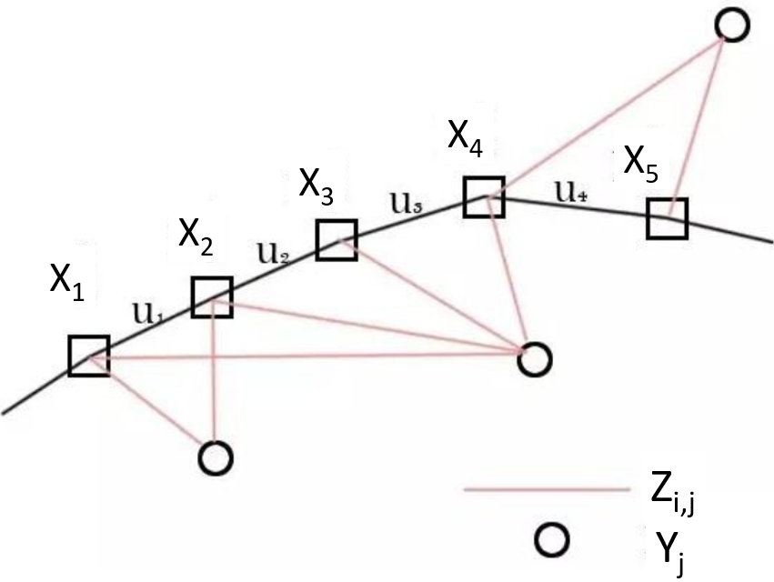
如下圖,我們藉由運動方程及觀測方程,在知道 $u_i$(感測器相對位姿變化)及 $z_{i,j}$(地標觀測數據 in local coordinate)的情況,估計 $x_i$(location, 感測器位姿 in global coordinate)及 $y_j$(map, 實際地標點 in global coordinate),也就是個定位 (location) 及建圖 (map) 的問題。
Location (global coordinate): $\quad x_{i}, i=1, \ldots, n$ Landmarks (global coordinate): $\quad y_{j}, j=1, \ldots, m$
Motion equation (global coordinate): $\quad x_{i+1}=f\left(x_{i}, u_{i}\right)+w_{i}$ Observations equation (local coordinate): $\quad z_{i, j}=h\left(x_{i}, y_{j} \right) + v_{i, j}$
注意因爲 camera 視角和遮蔽的關係, $z_{i,j}$ 並非對所有 $(i,j)$ 都觀察的到 -> sparse graph!
vSLAM分成幾個部分:
-
Front End, 通常稱爲 tracking thread: Visual Odometry (VO) or Visual Inertial Odometry (VIO) :特徵提取和匹配,以及估計相鄰畫面(圖片)間感測器的的運動關係。具體說就是從兩張相鄰畫面計算 camera 的位姿變化: $z_{i,j}, z_{i+1, j} \to u_i$。
-
Back End, 通常稱爲 mapping thread: Pose Estimation/Optimization:透過狀態 (states) 來表達自身及環境加上噪聲的不確定性,並採用濾波器或圖優化去估計狀態 (estimate states) 的均值和不確定性。就是從多張畫面估計 camera 位姿和地標:$z_{i,j}, u_i \to x_i, y_j$
-
Closed Loop Detection,透過感測器能識別曾經來到過此地方的特性,解決隨時間漂移的情況;
Visual Odometry (VO): tracking
包含兩個部分:(i) 定義 $y_j$ : 就是 feature extraction and matching (特徵提取和匹配);(ii) 估計相鄰畫面間感測器的的運動關係。具體說就是從兩張相鄰畫面計算 camera 的位姿變化: $z_{i,j}, z_{i+1, j} \to u_i$, 6 DOF for 3D, 3 DOF for 2D。
有時候再加上使用 IMU 找出 $u_i$, 結合 VO 就稱爲 VIO.
Pose Optimization
就是從多張畫面估計 camera 位姿和地標:$z_{i,j}, u_i \to x_i, y_j$
兩種做法:Kalman filter or (Graph) optimization
Kalman Filter (微分法)
就是把 state space model 綫性化: \(\mathbf{x}_{k}=\mathbf{F}_{k} \mathbf{x}_{k-1}+\mathbf{B}_{k} \mathbf{u}_{k}+\mathbf{w}_{k}\)
\[\mathbf{z}_{k}=\mathbf{H}_{k} \mathbf{x}_{k}+\mathbf{v}_{k}\]where
- $\mathbf{F}{k}$ is the state transition model which is applied to the previous state $\mathbf{x}{k-1}$;
- $\mathbf{B}{k}$ is the control-input model which is applied to the control vector $\mathbf{u}{k}$;
-
$\mathbf{w}{k}$ is the process noise, which is assumed to be drawn from a zero mean multivariate normal distribution, $\mathcal{N}$, with covariance, $\mathbf{Q}{k}: \mathbf{w}{k} \sim \mathcal{N}\left(0, \mathbf{Q}{k}\right)$.
- $\mathbf{H}_{k}$ is the observation model, which maps the true state space into the observed space and
- $\mathbf{v}{k}$ is the observation noise, which is assumed to be zero mean Gaussian white noise with covariance $\mathbf{R}{k}$ : $\mathbf{v}{k} \sim \mathcal{N}\left(0, \mathbf{R}{k}\right) .$
如果 noises 都是 normal distribution. 最佳的 solution 就是 Kalman filter.
Optimization (變分法)
-
From sensor: $z_{i,j}, u_{i}$
-
And Initial Guess: $\bar{x}{i}, \bar{y}{j}$
-
Then, we can estimate errors from motion and observation equations (P 代表 pose, L 代表 Landmark) \(e_{i}^{P}=\bar{x}_{i+1}-f\left(\bar{x}_{i}, u_{i}\right), e^{L}_{i, j}=z_{i, j}-h\left(\bar{x}_{i}, \bar{y}_{j}\right)\)
\[\min \varphi_{x_i, y_j}=\sum_{i}\left(e_{i}^{P}\right)^{2}+\sum_{i, j}\left(e^{L}_{i, j}\right)^{2}\]
這是 Nonlinear least square optimization
-
優化的方法: 2nd order method 用到 Jacobian 和 Hessian。此處的 $\mathbf{x} = (x_i, y_j)$ \(J=\frac{\nabla \varphi}{\nabla \mathbf{x}}, H=\frac{\nabla^{2} \varphi}{\nabla \mathbf{x} \nabla \mathbf{x}^{T}}\)
注意 $J$ and $H$ 是 sparse matrix 或是 sparse graph.
Method 1: Newton-Gauss method: 也是 linearized cost function, 再用 linear least square optimization iterative 解。注意這是 sparse matrix.
Method 2: Graph optimization or Bundle adjustment
由於優化的稀疏性,人們喜歡用“圖”來表達這個問題。所謂圖,就是由節點和邊組成的東西。我寫成G={V,E},大家就明白了。V是優化變量節點,E表示運動/觀測方程的約束。更糊塗了嗎?那我就上一張圖。
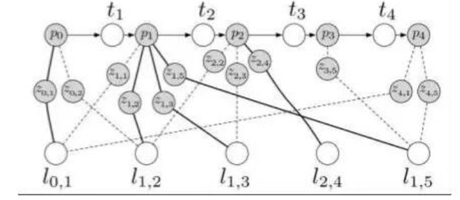
上圖中,p (=x) 是機器人位置,l (=y) 是地標,z 是觀測,t (=u) 是位移。其中呢,p, l (x,y) 是優化變量,而 z,t (z, u) 是優化的約束。看起來是不是像一些彈簧連接了一些質點呢?因為每個路標不可能出現在每一幀中,所以這個圖是蠻稀疏的。
不過,“圖”優化只是優化問題的一個表達形式,並不影響優化的含義。實際解起來時還是要用數值法找梯度的。這種思路在計算機視覺裏,也叫做Bundle Adjustment。