Introduction
AI for AI: use github Copilot for general signal processing, plotting, and machine learning.
Python Copilot
結論:Copilot 對一般的 python programming 初步看起來不錯。對於 machine learning 部分還要再測試。
Get Max and Min of a list
非常容易,參考 reference
A Simple Calculator
非常容易,參考 reference
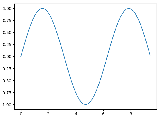
Plot a sine wave
只要 type ‘'’plot a sine wave using matplotlib’’’, 就會 generate the following code and work!!!
1 | |
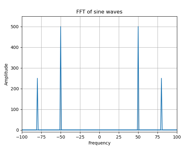
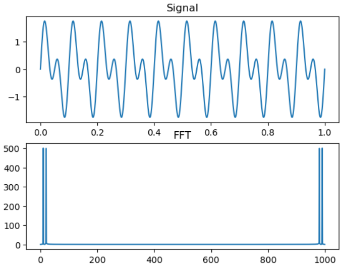
Compute a FFT of a sine wave and plot
Type ‘'’compute fft of a signal and plot it’’’, 就會得到以下的 FFT 以及 plot in linear or log scale!
1 | |
Classification (MNIST)
是否可以用 copilot for image classification? Yes, need more exploration.
Use Pytorch as example
use [ctl-enter] to view all examples!
Start with comment: ‘’’ mnist example using pytorch’
First import all packages:
1 | |
再來是煉丹五部曲!
Step 1: load dataset, type: def load_dataset => return mnist train_loader, test_loader!
1 | |
Step 2: build a model: type : class resnet
1 | |
Step 3: train a network: type def train
1 | |
Step 4: test a trained network: type def test
1 | |
Julia Copilot
用幾個常見的例子。
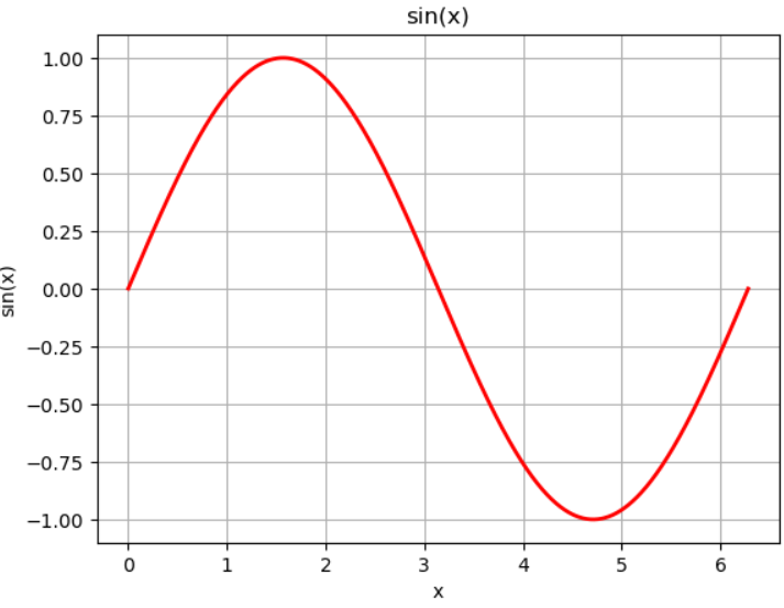
Plot a sin wave
Type “plot a sine wave”
1 | |
Results: failed.
Problem and fix.
- Still use old Julia code not working: linspace(0, 2pi, 1000) -> range(0, 2pi; length=1000)
- No vector operation: y = sin(x) -> y = sin.(x)
- Figure not display! Add display(gcf())
修改的版本 and work.
1 | |
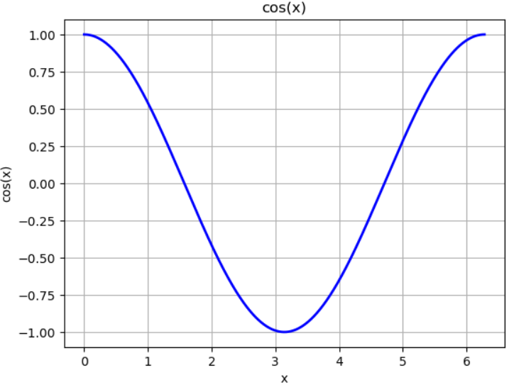
不過我再 type: plot a cosine wave, Copilot 可以現學現賣!
1 | |
Compute and Plot FFT
再 type “compute the FFT of a signal and plto the result”. 還是不行!
1 | |
-
Problem and fix.
- linspace(0, 2pi, 1000) -> range(0, 2pi; length=1000)
- No vector operation: sin(x) -> sin.(x); abs(x) -> abs.(x)
- plot -> PyPlot.plot
- Figure not display! Add display(gcf())
修改的版本 and work.
1 | |
Compute and Plot Self Entropy
基本上 input title 和 input signal range. Copilot 自動 show 出 entropy 的 formula in vector form!
1 | |
