Introduction
Entropy (熵) 是物理中非常重要但又很難抓住的觀念。似乎只有巨觀或是統計的定義,缺乏微觀或是第一性原理。
常見的説法是亂度。熱力學定律亂度會隨時間增加,因此一個對時間方向(過去、現在、未來)的觀察就是用亂度增加來定義。微觀的物理定律基本都是對時間方向對稱,沒有對應 entropy 的觀念。Entropy 似乎存在巨觀或是統計的定義。
Shannon 在二十世紀給 information 一個石破天驚的定義,就是 entropy. 這個定義把物理的熱力學、統計力學和 information/communication/data science 連結在一起,非常了不起的發現和洞見。
**基本 entropy 和 information 可以互換。另外所有的 entropy (self/conditional/cross) 和 information (Shannon/Fisher/mutual) 都是正值 (Wrong! discrete RV 都是正值。Continuous RV 有可能負值,不過是少數例外的情況。) **
Q1: Maximum likelihood estimation (MLE) and maximum mutual information (estimation?) 是同樣的事?或是同等的觀念只是不同的 objectives?
Ans: **No. MLE 是針對 “parameter” estimation. Maximum mutual information (i.e. joint-entropy) 比較類似 maximum entropy principle 是針對 distribution 的 constraint 或者更精確是 “bound”. ** 例如:
-
Maximum entropy principle: given a fixed variance $\sigma^2$, Normal disribution $N(\mu, \sigma^2)$ 有最大的 entropy (bound)!. 注意 entropy or information 基本是 mean independent. 也就是無法做為 mean parameter estimation! (unlike MLE)
-
Noisy channel information theory: given a noisy channel (e.g. additive noise with noise $\sigma^2$ 或是 binary nose channel with probabiliy $p$ to make mistake). Maximum mutual information principle 提供 channel capacity, 就是如何 reliably communcate without error! 但並沒有說如何每一個 bit 如何 estimate 是 0 or 1。比較是一個 bound (constraint).
-
如果給一堆 (random) samples, MLE 是要從這堆 samples 估計出一個 given underline distribution 的 parameter (mean, variance, etc.). Maximum entropy or joint-entropy (or cross-entropy) 則是提供一個 “bound” to approach?
-
How about minimize cross-entropy loss? the same concept? 當我越接近這個 bound, 我越接近 true distribution? 或是抓到真正的 feature distribution? Yes!! 如同 self-entropy case, 如果越接近 maximum entropy bound, distribution 越接近 normal distribution? 比較間接方法得到一個 “distribution”, not a parameter!
-
舉例而言,一個 noisy communication channel, MLE 是每一個 bit 如何估計是 0 or 1. Maximum mutual information principle 提供 channel capacity, 就是如何 reliably communcate without error! 但並沒有說如何每一個 bit 如何 estimate 是 0 or 1。比較是一個 bound (constraint).
-
當然 MLE 在 Bayesian 也變成 distribution estimation instead of parameter estimation. (Max) Information or (Min) cross-entropy 也可以用來 constraint/bound the distribution, 兩者也變的相關或相輔相成。(self, mutual, conditional?) information 應該無法 estimation mean; 但是 cross-entropy 則和 mean 相關,好像可以用來 estimate mean? Relative entropy = self-entropy + KL divergence (cross-entropy?)
Q2: The difference between (statistics) communication estimation theory and machine learning theory.
Q2b: how the PCA vs. mutual information at feature selection?
Ans:
Q3: Relative entropy is the same as KL divergence (sort of geometric meaning of distance between two distribution). What is cross entropy physical or geometric meaning?
Ans:
Shannon Information : (Self)-Entropy
分成 continuous variable or discrete random variable.
Discrete Random Variable
Self-entropy 的定義如下 \(\mathrm{H}(X)=-\sum_{i=1}^{n} \mathrm{P}\left(x_{i}\right) \log \mathrm{P}\left(x_{i}\right)\) 幾個重點:
- 因為 $\sum_{i=1}^{n} \mathrm{P}\left(x_{i}\right) = 1$ and $1\ge \mathrm{P}(x_{i})\ge 0$, 所以 discrete RV 的 entropy $H(X) \ge 0$. (注意,continuous RV 的 entropy 可能會小於 0!)
- Log 可以是 $\log_2 \to H(x)$ 單位是 bits; 或是 $\log_e \to H(x)$ 單位是 nat; 或是 $\log_{10} \to H(x)$ 單位是 dits.
Continuous Random Variable
Self-entropy 的定義如下 \(\mathrm{H}(X)=-\int p\left(x\right) \log p\left(x\right) d x\) 幾個重點:
- 因為 $\int p\left(x\right) d x = 1$. 重點是 $p(x) \ge 0$ , 但 $p(x)$ 可以大於 1. 所以注意,continuous RV 的 entropy 可能會小於 0!
- Log 可以是 $\log_2 \to H(x)$ 單位是 bits; 或是 $\log_e \to H(x)$ 單位是 nat; 或是 $\log_{10} \to H(x)$ 單位是 dits.
Example 1: Entropy of a uniform distribution, X ∼ U(a, b)
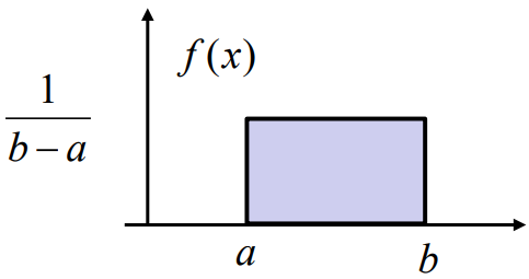
$H(X) = \log (b-a)$
Note that $H(X) < 0$ if $(b-a) < 1$
Example 2: Entropy of a normal distribution, $X \sim N(\mu, \sigma^2)$
\[H(X) = \frac{1}{2}\ln (2\pi e \sigma^2) = \frac{1}{2}\ln (2\pi \sigma^2) + \frac{1}{2} \label{entNormal}\]Note that $H(X) < 0$ if $2\pi e \sigma^2 < 1$, entropy 和 mean 無關,只和 variance 相關。
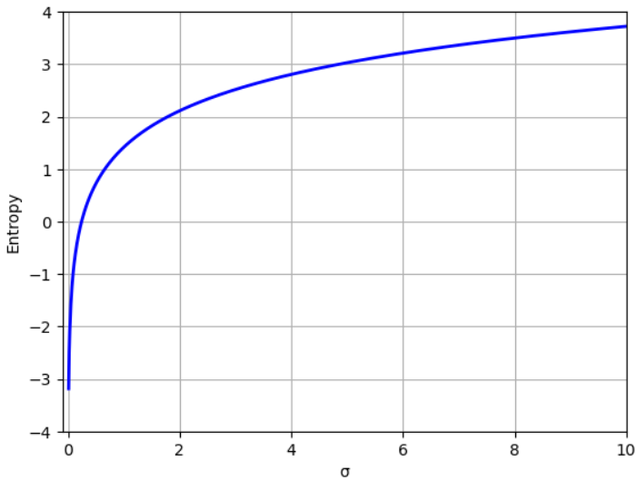
Maximum Entropy Theory
這是一個常用的理論:Given a fixed variance, maximum entropy distribution 是 normal distribution (independent of mean).
因此 normal distribution 的 entropy 也就是 entrropy 的 upper bound!!, 如上圖。
Self-Entropy Summary
Entropy 是衡量一個 distribution 的亂度或資訊量 (通常大於 0): Distribution $\to$ Scaler (>0). Maximum entropy theory 則是 given 一個 scaler ($\sigma^2$), 找出最大 entropy 的 (normal distribution), 其實就是 Scaler (>0) $\to$ Distribution
Entropy/information 基本和 distribution 的 mean 無關。 如果是 normal distribution, $\eqref{entNormal}$ 告訴我們 entropy/information 和 variance 是一對一的關係。從 entropy 可以完全決定 distribution (除了 mean 之外)。
初步直覺,maximum entropy 也許可以用來 estimate variance 之類的 parameter, 但無法 estmate mean. 因此 in general maximum entropy 和 maximum likelihood estimation 是不同的東西。
XYZ-Entropy
一個隨機變數 (RV) 的 distribution 沒有太多的變化。接下來我們考慮兩個隨機變數相關的 entropy/information.
我們先看幾個例子
Noisy Channel (Estimation)
| 在 communication 或是 storage 常常見到這類問題。Source (Z) 是 hidden state, 一般是 binary 0 or 1. Channel 可以是 additive noise channel 或是 binary noisy channel. Output (X) 是 observation (evidence),可以是 continuous 或是 binary. 數學上一般用 $p(x | z)$ 表示。 |
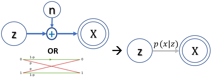
一般 (X, Z) 有 correlation, 或者是 mutual information. 這是一類問題,計算 channel capacity,就是這個 channel 能送多少 information reliably. Mutual information 是一個 global 概念,不是用個別 X or Z sample 的問題。
另一類問題是從個別 X estimate 個別 Z. 這是 estimation problem.
- Maximum Likelihood Estimation (MLE), why not MAP? MAP is biased (by the prior distribution)!
In turn of information theory => find the maximum mutual information between (X, Z): overall channel capacity, not individual X.
Is Maximum Log-Likelihood Estimation this same as Maximum Mutual Information??? : NO
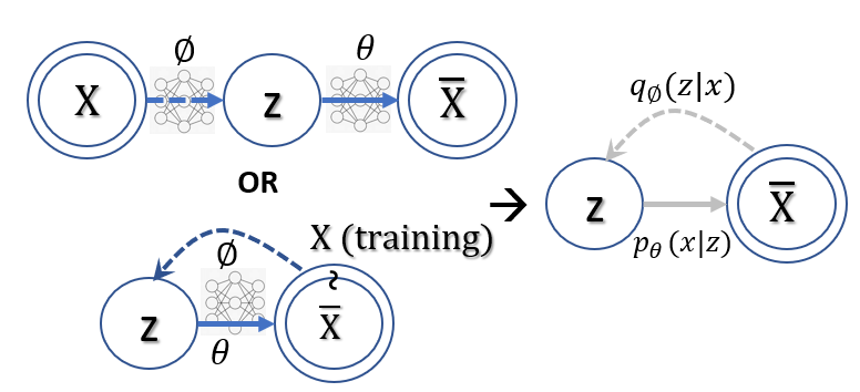
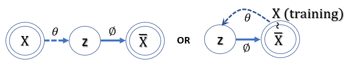
In machine learning such as VAE. 問題不同!
Macine Learning VAE 的 goal: (1) Maximize the mutual information of (X input, Y output) ! (2) Maximize the hidden variable (z, at the middle) 的 self-information! (regularization)
Why? 如果 ML 只是 maximize mutual information of (X, Y) => 就讓 Y = X 就 OK! 顯然不是我們要的,因爲在 training 才有 X; 在 inference (or generation) 沒有 X, 需要從 Z (hidden variable) 產生 Y!
所以目標變成 maximize the mutual information of (X, Y) and mzximize the self-entropy of hidden variable Z (Gaussian) during training. 這樣在 inference 時才能保證 (z, X_bar) has the maximum mutual information?
Is PCA a maximum mutual information?
Relative entropy and cross entropy 非常類似!
-
測量兩個 (marginal) distributions 的相似程度,沒有任何測量兩個 distribution 的相關程度!也許這樣就夠了? for machine learning or deep learning with very high dimension? NO! See VAE 的推導,仍然等價與 VAE loss = -1 x mutual information + KL divergence of regularion term (KL(p(z)//q(z x)) -
一般是數學工具用於理論推導 (VAE) or formulation (cross entropy loss)
-
Statistics Communication 比較簡單,能夠控制的不多。目標就是 maximize mutual information of (X, Y)
- ML 可以通過使用 neural network 引入 regularization term? 除了 maximize mutual information (X, Y) 還要 balance regularization to make the hidden variable 是非常 simple (high entropy) distribution?
ML 的 goal: (1) Maximize the mutual information of (X input, Y output) ! (2) Maximize the hidden variable (z, at the middle) 的 self-information! (regularization)
Why? 如果 ML 只是 maximize mutual information of (X, Y) => 就讓 Y = X 就 OK! 顯然不是我們要的,因爲在 training 才有 X; 在 inference (or generation) 沒有 X, 需要從 Z (hidden variable) 產生 Y!
所以目標變成 maximize the mutual information of (X, Y) and mzximize the self-entropy of hidden variable Z (Gaussian)
=
Relative Entropy (~KL Divergence)
我們先從最簡單的 relative entropy (相對熵) 開始,等價於 KL (Kullback-Leibler) divergence, 其定義:
幾個重點:
-
KL divergence 永遠大於等於 0 (regardless discrete or continuous distribution)! 如果兩個 distribution 長得完全一樣,KL divergence = 0. 因此有時用來衡量兩個 distribution 的 “距離”。兩個問題:(1) KL divergence 不對稱 KL(P Q) <> KL(Q P) 和一般距離的概念不同;(2) KL divergence 完全沒有考慮兩個 distribution 的”相關性”。 -
KL divergence 只是測量兩個 (marginal) distributions 的相似程度,沒有任何測量兩個 distribution 的相關程度! 例如 P ~ N(0, 1), Q ~ N(0, 1) DKL(P Q) = 0 不論 P, Q 是完全 independent, 或是完全相關。因爲 KL divergence 不含 P, Q joint pdf 或是 P, Q conditional pdf. -
KL divergence 一般是數學工具用於理論推導。但是 P 或是 Q 可以是 conditional pdf, 如此 KL divergence (relative entropy) 可以衡量兩個distribution 的相關性! ( I(X; Y) = E{KL(P(X Y) P(X) ))}) -
Cross entropy = H(p) + KL(P Q)
Cross Entropy (Loss)
在資訊理論中,基於相同事件測度的兩個概率分布{\displaystyle p}

the other equation we need (using this new nn-normalized formulation) is the formula for cross-entropy. It is almost identical, but it compares two different probabilities: it gives us a way to measure the “cost” of representing one probability distribution with another. (Concretely, suppose you compress data from one distribution with an encoding optimized for another distribution; this tells you how many bits it will take on average.)
同樣 cross entropy 沒有考慮兩個 distribution 的相關性。只是 distribution 的形狀。
-
Cross entropy 也是不對稱。如果 q distribution 和 p distribution 完全一樣,則是 H(p, q) = H(p), 如果不一樣, H(p, q) > H(p) or H(p, q) - H(p) = KL(p q). 一般 machine learning 好像就是 minimize cross entropy loss. NO! still involve mutual information + regularization. - Minimize cross-entropy loss in a sense to minimize KL divergence of (p, q)? 爲什麽不直接 minimize relative entropy? 有 regularization 的意味嗎 ?
Conditional entropy, joint entropy (mutual information) 則是另一組。重點不是 distribution 的形狀,而是兩個 RV 的相關性!!! 主要用於 communication theory. recovery signal from noise.
Q: diffusion model for generative model?
Conditional Entropy, Joint Entropy (Mutual Information), Marginal Entropy,
In probability theory and information theory, the mutual information (MI) of two random variables is a measure of the mutual dependence between the two variables. More specifically, it quantifies the “amount of information” obtained about one random variable, through the other random variable.
Not limited to real-valued random variables like the correlation coefficient, Mutual Information is more general and determines how similar the joint distribution p(X,Y) is to the products of factored marginal distribution p(X)p(Y). Mutual Information is the expected value of the pointwise mutual information (PMI).


| H(X) = H(X | Y) + I(X; Y) |
| H(Y) = H(Y | X) + I(X; Y) |
| H(X, Y) = H(X) + H(Y | X) = H(Y) + H(X | Y) = H(X) + H(Y) - I(X; Y) |
I(X; Y) = H(X) + H(Y) - H(X, Y)
I(X;Y) ≤ H(X) and I(X;Y) ≤ H(Y)
可以證明: H(X), H(Y), H(X, Y), I(X; Y) ≽ 0
| 如果 X and Y 獨立。 I(X; Y) = 0, H(X | Y) = H(X), H(Y | X) = H(Y), H(X, Y) = H(X)+H(Y) |
如果 Y 完全 depends on X. I(X; Y) = H(X) = H(Y) = H(X, Y)

Cross Entropy
Cross Entropy & DL-divergence
Cross Entropy & Fisher Information
Fisher information
Fisher information and cross-entropy
VAE Loss Function Using Mutual Information
VAE distribution loss function 對於 input distribution $\tilde{p}(x)$ 積分。 $\tilde{p}(x)$ 大多不是 normal distribution.
\[\begin{align*} \mathcal{L}&=\mathbb{E}_{x \sim \tilde{p}(x)}\left[\mathbb{E}_{z \sim q_{\phi}(z | x)}[-\log p_{\theta}(x | z)]+D_{K L}(q_{\phi}(z | x) \| \,p(z))\right] \\ &=\mathbb{E}_{x \sim \tilde{p}(x)} \mathbb{E}_{z \sim q_{\phi}(z | x)}[-\log p_{\theta}(x | z)]+ \mathbb{E}_{x \sim \tilde{p}(x)} D_{K L}(q_{\phi}(z | x) \| \,p(z)) \\ &= - \iint \tilde{p}(x) q_{\phi}(z | x) [\log p_{\theta}(x | z)] dz dx + \mathbb{E}_{x \sim \tilde{p}(x)} D_{K L}(q_{\phi}(z | x) \| \,p(z)) \\ &= - \iint q_{\phi}(z, x) \log \frac{ p_{\theta}(x, z)}{p(x) p(z)} dz dx + \mathbb{E}_{x \sim \tilde{p}(x)} D_{K L}(q_{\phi}(z | x) \| \,p(z)) \\ \end{align*}\]對 $x$ distribution 積分的完整 loss function, 第一項就不只是 reconstruction loss, 而有更深刻的物理意義。
記得 VAE 的目標是讓 $q_\phi(z\mid x)$ 可以 approximate posterior $p_\theta(z\mid x)$, and $p(x)$ 可以 approximate $\tilde{p}(x)$, i.e. $\tilde{p}(x) q_{\phi}(z\mid x) \sim p_\theta(z\mid x) p(x) \to q_{\phi}(z, x) \sim p_\theta(z, x)$.
此時再來 review VAE loss function, 上式第一項可以近似為 $(x, z)$ or $(x’, z)$ 的 mutual information! 第二項是 (average) regularization term, always positive (>0), 避免 approximate posterior 變成 deterministic.
Optimization target: maximize mutual information and minimize regularization loss, 這是 trade-off.
\[\begin{align*} \mathcal{L}& \sim - I(z, x) + \mathbb{E}_{x \sim \tilde{p}(x)} D_{K L}(q_{\phi}(z | x) \| \,p(z)) \\ \end{align*}\]Q: 實務上 $z$ 只會有部分的 $x$ information, i.e. $I(x, z) < H(x) \text{ or } H(z)$. $z$ 產生的 $x’$ 也只有部分部分的 $x$ information. $x’$ 真的有可能復刻 $x$ 嗎?
A: 復刻的目標一般是 $x$ and $x’$ distribution 儘量接近,也就是 KL divergence 越小越好。這和 mutual information 是兩件事。例如兩個 independent $N(0, 1)$ normal distributions 的 KL divergence 為 0,但是 mutual information, $I$, 為 0. Maximum mutual information 是 1-1 對應,這不是 VAE 的目的。 VAE 一般是要求 marginal likelihood distribution 或是 posterior distribution 能夠被儘可能近似,而不是 1-1 對應。例如 $x$ 是一張狗的照片,產生 $\mu$ and $\log \sigma$ for $z$, 但是 random sample $z$ 產生的 $x’$ 並不會是狗的照片。
這帶出 machine learning 兩個常見的對抗機制:
- GAN: 完全分離的 discriminator and generator 的對抗。
- VAE: encoder/decoder type,注意不是 encoder 和 decoder 的對抗,而是 probabilistic 和 deterministic 的對抗 => maximize mutual information I(z,x) + minimize KL divergence of posterior $p(z\mid x)$ vs. prior $p(z)$ (usually a normal distribution).
(1) 如果 x and z 有一對一 deterministic relationship, I(z, x) = H(z) = H(x) 有最大值。但這會讓 $q_{\phi}(z\mid x)$ 變成 $\delta$ function, 造成 KL divergence 變大。 (2) 如果 x and z 完全 independent, 第二項有最小值,但是 mutual information 最小。最佳值是 trade-off result.
Reference
[1] Wiki, “Cross entropy”
[2] James Gleich, “The Information: A History, a Theory, a Flood”
[3] “Lecture 11 : Maximum Entropy”
[4] Wiki, “Maximum entropy probability distribution”
熵 = uncertainty = information (in bit)
Two PDFs in Communication
熵用在編碼和通訊請參見前文。對一個通訊系統包含兩個 probability distributions.
一個是 source probability distribution, 一個是 channel noise 形成的 channel probability distribution.
分別對應 H (source entropy) 和 C (channel capacity).
為了讓 source information 能夠有效而且無損的傳播,需要使用 source/channel encoder/decoder.

Go Fundamental
另一個更基本的觀點,輸入 (source) 是一個 probability distribution X, 通過 channel probability distribution Q,
得到輸出 probability distribution Y.

基本的問題是 X and Y 能告訴什麼關於 information 的資訊?
X and Y 的 probability 可以定義:
p(x): source probability
| p(y | x): conditional pdf, 其實就是 channel probability distribution Q |
| p(x, y) = p(x) p(y | x) |
p(y) = ∑x p(x, y)
對應的 entropy (or information) related:
H(x) = Ex(-log p(x)): source entropy or source information in bit
| H(y | x) = Ey | x(-log p(y | x)) : channel entropy 如果是 symmetric channel, 就和特定的 x 無關! |
| H(x, y) = Ex,y(-log p(x, y)) = Ex,y(-log p(x)) + Ex,y(-log p(y | x)) = H(x) + H(y | x) assuming symmetric channel! |
H(y) = Ey (-log p(y)) ≽ H(x) in cascaded structure (entropy always increase?!)
| 直觀而言,Q (p(y | x)) 的 entropy 愈小 (capacity ~ 1), p(y) ~ p(x). |
H(y) ~ H(x) (information preserve).
如果 Q 是 50%/50% probability distribution (capacity ~ 0), H(y) ~ 1-bit.
Output Entropy 增加,information 無中生有?
顯然 information 只看 output probability distribution 是無意義的。因為 entropy 一定愈來愈大。
直觀上 entropy/information 不可能無中生有。必須另外找 X,Y information 的定義。
Wrong explanation!
Channel noise 也有 entropy/information. Output information 包含 source 和 noise information. Information 並未無中生有。
| 我們要找的是和 input source 有關的 information, 就是 H(Y) - H(Y | X), output information 扣掉 channel noise/information. |
剩下的是和 input source 直接相關的 information (i.e. mutual information), 顯然 mutual information 一定等於或小於 input information.
Two Entropies in Communication
下圖清楚描述 entropies 在 communication 的變化。 X -> Y ; H(Y) ≽ H(X)

| I(X; Y) = H(Y) - H(Y | X) 是存留的 H(X) information after channel contamination H(X | Y). |
| 顯然 I(X; Y) depends on H(X) and H(Y | X); I(X; Y) 可視為 information bottleneck or channel capacity. |
| H(Y | X) 是由 channel noise model 給定。所以 channel capacity 由 Px(x) 決定。 |
Channel capacity 的定義:

| C = sup I(X; Y) = sup [ H(Y) - H(X | Y) ] = sup [ H(Y) - Hb ] = 1 - Hb (proof) |

The channel capacity of the binary symmetric channel is
where {\displaystyle \operatorname {H} _{\text{b}}(p)}
Two PDFs in Encoding
Cross Entropy (交叉熵)
In information theory, the cross entropy between two probability distributions
measures the average number of bits needed to identify an event drawn from the set, if a coding scheme is used that is optimized for an “unnatural” probability distribution
幾個重點:
\1. p and q 都是 probability distribution 而且 over the same set of events (或是 same discrete classes for machine learning).
\2. 假設 p 是 true distribution, cross entropy H(p, q) 代表 q distribution 和 p 的距離?No, that is KL divergence.

-log q 顯然不是真的 information. -log q ≽ 0, 所以 H(p, q) = Ep(-log q) ≽ 0, H(p, q) ≠ H(q, p)
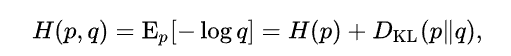
| H(p, q) = H(p) + D(p | q), where H(p) 是 true information, D(p | q) 是 KL divergence ≽ 0 |
| D(p | q) 就是冗余。 H(p, q) = H(p) (true information) + D(p | q) (冗余) |
H(p, q) ≽ H(p) 但是 H(q) 不一定大於 H(p). 因為 q distribution 可以任意選,說不定選的 q 的 H(q) 小於 H(p).
但是 H(p, q) 永遠大於等於 H(p), 多出的部分就是冗余。
For example, 英文有 26 字母。出現的統計特性不同,一般 ‘e’ and ’t’ 有非常高的頻率。’z’ 又很低的頻率。
假設 “true” distribution p 是 32-bit 的 Binomial distribution, H(p) = 3.55-bit
假設 q distribution 是 32-bit uniform distribution, H(q) = 5-bit
| H(p, q) = H(p) + D(p | q) = 3.55 + ?? = - sum { p(x) log 1/32 } = 5-bit |
| D(p | q) = 5 - 3.55 = 1.45 bit 就是冗余 |
if p = q, same distribution H(p, q) = H(p) = H(q)
if q is a uniform distribution, H(p, q) = - log q(x) = n for 2^n outcomes.
注意 if q 是 uniform distribution, H(p, q) = H(q) = n 是和 p (true distribution) 無關!
但若 q 不是 uniform distribution, H(p, q) ≠ H(q)
如果沒有 prior knowledge of true distribution p. 最直接的方法是選 q 為 uniform distribution.
H(p, q) = H(q) = n, H(p) 一定小於等於 H(p, q). 多出的部分是冗余,可以之後由 posterior data infer.
Relative Entropy (相對熵)
Relative entropy (相對熵) 是和 cross entropy (交叉熵) 非常相似而且容易混淆的名詞。
Relative entropy 就是 Kullback-Leibler divergence, 用來測量兩個 PDFs 的相似程度。

| 如果 P and Q PDFs 長的完全一樣。D(P | Q) = 0. 可以證明 D(P | Q) ≽ 0. |
| H(p, q) = H(p) + D(p | q) |
=> Cross entropy = “true” entropy + relative entropy or 交叉熵 = “真“ 熵 + 相對熵
Two PDFs in Summary
Two PDFs (p and q) 有兩種可能情況:
(1) over two different sets of events,或是說兩個 random variables, X, Y 各自的 distributions, p(x) and q(y).
由此可以定義 X, Y 的 mutual information,I(X;Y), 就是 X, Y information 交集(或相關)的部分。
I(X; Y) ≤ H(X) or H(Y)
如果 X 和 Y 有因果關係;例如通訊系統 X 是 transmitted signal, Y 是 received signal. 或是在 storage system,
X 是 stored signal, Y 是 read out signal. 可以定義 channel capacity C = sup I(X; Y) over all p(x).
| 一般而言 p(x) 是 uniform distribution (max H(X)) 而且 p(y | x) 是 symmetric, 會有 max I(X; Y). |
可以想像 I(X; Y) 成 p and q 是 topology 某種串聯。但 mutual information 卻變小。(不要想 resistance, 想 conductance).
(2) over same set of event, 就是同一個 random variable 卻有兩個 distributions. 顯然一個, p(x), 是 true distribution;
q(x) 是近似 distribution 或是 initial guessing distribution. 此時可以定義 cross entropy H(p, q) = H(p) + DL(p//q)
代表 approximate distribution 和 true distribution 的 information 的關係。注意是 true information (in bit) 加上冗余 information (in bit).
H(p, q) ≽ H(p) ,但 H(p, q) 或 H(p) 不一定大於或小於 H(q)
可以 H(p, q) 想像成 p and q 是 topology 某種並聯。但 cross entropy 卻變比 H(p) (but not necessary H(q)) 大。
乍看冗余是壞事,在 (2) 我們希望冗余愈小愈好,最好是零。這正是 source encoder 做的事 (source encoding or compression).
事實並非如此。參考[2], 冗余在 noisy channel, 也就是 (1) 的情形,有助於達到 error free communication. 這在日常口語很常見。
即使部分的聲音沒聽清楚,我們還是可以根據上下文判斷正確的意思。
重點是最少要加多少冗余,以及如何加冗余。這正是 channel encoder 做的事。
Shannon-Hartley 告訴我們 channel capacity 和 SNR and Bandwidth 的關係。但是並未告訴我們如何加冗余。
(間接)可以算出最少加入冗余 (error correction code),使通訊系統有機會達到 Shannon channel capacity without error.
Example:
H(source) = 1-bit C = 0.5-bit 根據 Shannon-Hartley theorem 是無法達到 error free communication.
如果 code rate 1/3 (e.g. LDPC)
H’(source) = 1-bit C’ = 1.5-bit 有機會達到 arbitrary low error rate.
下圖顯示 output signal y = x + noise 的 H(y) > H(x). 在 output 之後需要加上一個 decoder block.
Decoder 的目的是從 y 得到 x’, 而且 x’ = x. 用數學表示
H(x’) = H(x) < H(y) 同時 I(x’, x) = H(x)
從熱力學角度來看,decoder 是做減熵同時又要回到和 source 一樣的 mutual information. (reverse the process)
這是需要付出代價,就是“做功”。 Decoder 直觀上需要“做功”才能達到減熵的效果。
Decoder complexity 相當於“做功”。 Kolmogorov 的 algorithmic information theory 就是在處理這個部分。
即使在熱力學也有類似的問題:Maxwell demon 也是用 computation or algorithm 減熵。
當然 total system entropy (including the computation) always increase. 沒有違反熱力學第二定律。
Two PDFs in Machine Learning
機器學習或是深度學習是熱門題目。結合 learning 和 information theory 的相關 papers 車載斗量。
似乎不若 communication 或是 coding theory 有簡單而深刻的結論。有一些有用的技巧如下。
Cross Entropy or Relative Entropy Minimisation (Optimization)
Cross entropy or relative entropy can be used to define the loss function in machine learning optimization.
The true probability {\displaystyle p_{i}}

在分類問題 (classification) 大多的情況沒有 “true probability distribution”, 只有 (truth) label samples, {0, 1} or multiple classes with (one-shot) label.
Predicted probability 通常由 logistic function 或是 neural network 產生,目標是儘量接近 true probability distribution.
| 有兩個方法:(1) minimize relative entropy or KL divergence D(p | q); or (2) minimise cross entropy H(p, q) = H(p) + D(p | q). |
如果 p 是 “true probability distribution”, H(p) 可視為常數。(2) 和 (1) 基本等價。
常見的 binary classification 可以用 minimise “cross entropy loss” 達成。

| Cross entropy 和 relative entropy 完全相同因為 H(p=0) = H(p=1) = 0, H(p, q) = D(p | q) |
y^ 通常由 logistic function 計算得出:

Cross entropy loss function 定義 cross entropy 的 sample average.

如果 y=1: -[y log y^ + (1-y) log (1-y^)] 如下圖。如果 y=0: 下圖左右鏡射。 J(w) 就是很多這樣的 loss function 平均的結果。
J(w) ≽ 0

Given y^ = 0.9
if y = 1
BCE loss = -1 * [ 1 * log 0.9 + 0 * log 0.1 ] = - log 0.9 = +0.15 (in bit)
if y = 0
BCE loss = -1 * [ 0 * log 0.9 + 1 * log 0.1 ] = - log 0.1 = +3.32 (in bit)
Question:
y^ 是否有可能收斂到 0 and 1? 或是 J(w) 收斂到 0? Yes, if samples are separable in binary classification.
想像 1D logistic regression, 如果 samples 是 binary separable, w (weight factor) 可以是無窮大,g(z) 就會是 0 or 1.
| 如果 y^ = g(z) 正確 training 到 y (0 or 1), H(y, y^)=D(y | y^)=H(y)=J(w)=0 (no information in samples since it’s already labelled) |
實務上會加上 regularisation term L2 norm of x 避免 overfitting. 因此 y^ 不會收斂到 0 and 1. J(w) always larger than 0.
One-hot category (more than binary class) classification 也可以用 minimise “cross entropy loss” 達成。
同樣 cross entropy:

y,’ 是 true label {0, 1} in K class. Cross entropy 完全相等於 relative entropy (KL divergence) 只要是 one-hot.
yi 是 softmax function (logistic function 的推廣)計算得出。

單一 sample cross entropy: -[ 0* log(0.3) + 0* log(0.25) + 1*log(0.45)]
Cross entropy loss function 同樣是 cross entropy 的 sample average.
Maximal Entropy Principle (Convex Optimization)
熱力學告訴我們宇宙 (或 close system) 的熵總是增加。
如果不知道 probability distribution, 就用 maximum entropy principle [4] 求得 probability distribution.
一般情況會有 constraints/prior information.
例如英文字母的機率分佈的 constraint 是 bounded 26 個字母。
Maximum entropy distribution for bounded constraints (discrete or continuous) is uniform distribution [4].
Maximum entropy distribution for fixed mean and variance is normal distribution [4].
Maximum entropy distribution for a fixed average kinetic energy (fixed T, temperature) is Maxwell-Boltzmann distribution.
Maximal entropy optimization 有一個很大的優點:entropy function 是 concave function. 可以用 convex optimization.
Entropy in Machine Learning
Maximal entropy optimization
Probability —> information by Shannon
How about Algorithm? (coding theory) —> information? by Komologov?
coding theory —> complexity theory —> information??
Analogy between thermodynamics and information theory