Takeaway
正規化包括四個參數:平均值 ($\mu$)、方差 ($\sigma^2$)、增益 ($\gamma$) 和偏差 ($\beta$)。平均值和方差是在數據上計算的統計信息,分別代表中心趨勢和變異性。增益和偏差是應用於正規化數據的可學習參數,允許模型在訓練過程中調整正規化過程。
-
平均值和方差是在 forward path 計算或是統計得到,不是 learnable parameters.
-
增益和偏差實在 backward path 調整的 learnable parameters.
機器學習正規化
正規化的重要性
正規化是機器學習模型訓練過程中的一個關鍵步驟。它在確保訓練過程的收斂性和效率方面發揮了重要作用。正規化有助於解決輸入特徵不均勻尺度的問題,確保模型更快地收斂並取得更好的性能。讓我們探討不同類型的正規化技術及其在增強機器學習模型訓練中的作用。
正規化将数据的各种特征缩放成一个共同的范围,通常在 0 到 1 之间,或者平均值为 0、标准差为 1。这样做有几个重要的优点:
- 改善收敛: 通过将特征缩放到相似的尺度,您可以确保每个特征对学习过程做出平等的贡献,使模型更快地收敛,并避免诸如梯度消失或爆炸等问题。
- 增强鲁棒性: 正規化减少了来自具有显著不同尺度的特征的异常值和偏差的影响。这会产生更鲁棒的模型,能够更好地泛化到未见过的数据。
- 防止数值不稳定: 在某些优化算法中,正規化可以防止由于特征之间幅度差异过大而引起数值不稳定,从而提高训练稳定性。
正規化的類型
在深度學習中,特別是在卷積神經網絡(CNNs)中,張量 (Tensor)是表示數據流入網絡的多維矩陣。張量中維度的順序通常遵循 (Batch, Channel, Height, Width)(批次大小,通道數,高度,寬度)的慣例,通常被稱為 Pytorch BCHW 格式。Tensorflow 則是用 BHWC 格式。讓我們分解每個維度:
- 批次大小(B)
- 代表一批中的樣本數或數據集的數量。在訓練過程中,模型通常在數據批次上進行訓練,以提高效率和泛化性能。
- 通道數(C)
- 對應於每個數據集中通道或特徵的數量。以影像爲例:
- 在灰度圖像中,通道數為1。
- 在RGB彩色圖像中,通道數為3(紅,綠,藍)。
- 在神經網絡的中間層等更復雜的情況下,通道數可以表示不同的學習特徵 3->8->16->32->64->128->256。
- 對應大語言模型 (transformer) 為例:
- 對應每個 embedding (由 token 查字典得來) 的維度,在 attention layer 注重在 embedding 之間的通訊,基本沒有 channel 計算,做多是 split 和 concatenate,像是 embedding dimension 和 multihead head dimension。在 FF layer,則注重在 channel 計算。
- 對應於每個數據集中通道或特徵的數量。以影像爲例:
- 高度(H)和 寬度(W),合稱為 Instance (or Vector)
- 以圖像爲例:H 代表高度,W 代表寬度,通常與圖像中的行數維度和列數維度相關。
- 以語言爲例:Instance 代表序列數據中的時間維度相關聯。
- 高度(H)和 寬度(W)和全部通道 (C),合稱為 Layer (or Tensor): 注意 R, G, B 不是三個 layers, 而是一個 layer/tensor.
- 高度(H)和 寬度(W)和部分的通道 (C),合稱為 Group
例如,如果有一批RGB圖像,尺寸為32x32,批次大小為16,張量形狀將是(16,3,32,32)。每個樣本有3個通道(RGB),每個通道有32個像素的高度和32個像素的寬度。
如果有一批語言,批次為 32, context length是 1024, embedding 是 768, 張量形狀將是 (32,768,1024)。
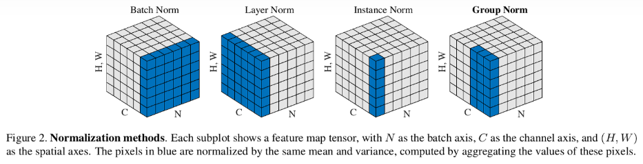
不同的正規化對應到不同維度縮放到標準分佈 (mean = 0, std = 1) :
圖像的正規化如下圖:
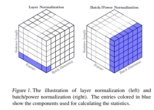
語言模型的正規化如下圖:注意 layer normalization 的定義不包含 sequence (i.e. time) dimension! 但是 batch normalization 卻是包含 sequence dimension.
放在一起:
Batch Normalization (BN)
批次正規化是由 Google 的 Ioffe 和 Szegedy 於 2015年提出的一種技術,它通過調整和縮放激活值來對每一層的輸入進行正規化。在深度神經網絡中,尤其在解決內部協變量漂移問題方面,這是一個特別有用的技術。
Batch Normalization (BN) 有兩個可能的局限性:
- BN 使用批次統計量: 對應於當前小批量的均值和標準差。然而,當批量很小時,樣本均值和樣本標準差不能很好地代表實際分佈,網絡無法學習到有意義的內容。
- 由於 BN 依賴批次統計量進行正規化,因此它較不適合序列模型。這是因為在序列模型中,我們可能有不同長度的序列,以及與更長序列相對應的更小批量大小。
接下來,我們將檢查層正規化,這是另一種可用於序列模型的技術。對於卷積神經網絡(ConvNets),仍建議使用批次正規化以實現更快的訓練。
Layer Normalization
層正規化是由 Lei Ba、Kiros 和 Hinton 於 2016年提出的。與批次正規化不同,它為每個樣本個別計算正規化統計信息,適用於具有不同輸入分布的任務。
Batch Normalization (BN) is widely adopted in CV, but it leads to significant performance degradation when naively used in NLP. Instead, Layer Normalization (LN) is the standard normalization scheme used in NLP.
Instance Normalization
實例正規化是由Dmitry Ulyanov、Andrea Vedaldi 和 Victor Lempitsky 於2016年提出的。它為每個實例(或樣本)獨立地在空間位置上對每個通道進行正規化,通常應用於風格轉移和圖像生成任務。
Group Normalization
群組正規化是由Yuxin Wu和Kaiming He於2018年提出的一種替代批次正規化的技術。它將通道劃分為群組並為每個群組獨立計算正規化統計信息,適用於批次大小較小的場景。
包含4個參數的正規化:平均值、方差、增益和偏差
正規化包括四個參數:平均值 ($\mu$)、方差 ($\sigma^2$)、增益 ($\gamma$) 和偏差 ($\beta$)。平均值和方差是在數據上計算的統計信息,分別代表中心趨勢和變異性。增益和偏差是應用於正規化數據的可學習參數,允許模型在訓練過程中調整正規化過程。
言簡意賅
- 平均值和方差是在 forward path 計算或是統計得到,不是 learnable parameters.
- 增益和偏差實在 backward path 調整的 learnable parameters.
計算流程
以 batch normalization 爲例:[@shenPowerNormRethinking2020]
下表非常好 summarize 整個流程,包含 training 的 forward and backward, 以及 inference forward.
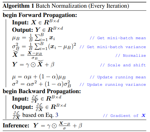
Input: Values of $x$ over a mini-batch: $\mathcal{B}=\left{x_{1} \ldots x_{m}\right}$; Parameters to be learned: $\gamma, \beta$
$\mu$, $\sigma$, $\gamma$, $\beta$ 的維度是和 channel 維度一致。
以影像爲例:(RGB) 各有一個 ($\mu$, $\sigma$, $\gamma$, $\beta$ ) , 而不是 share 用一組。
以語言 MLP linear + ReLu 爲例: 每一個 hidden node 都有一組
Output: $\left{y_i=\mathrm{BN}_{\gamma, \beta}\left(x_i\right)\right}$ \(\begin{aligned} & \mu_{\mathcal{B}} \leftarrow \frac{1}{m} \sum_{i=1}^m x_i \quad \text { // mini-batch mean } \\ & \sigma_{\mathcal{B}}^2 \leftarrow \frac{1}{m} \sum_{i=1}^m\left(x_i-\mu_{\mathcal{B}}\right)^2 \quad \text { // mini-batch variance } \\ & \widehat{x}_i \leftarrow \frac{x_i-\mu_{\mathcal{B}}}{\sqrt{\sigma_{\mathcal{B}}^2+\epsilon}} \quad \text { // normalize } \\ & y_i \leftarrow \gamma \widehat{x}_i+\beta \equiv \operatorname{BN}_{\gamma, \beta}\left(x_i\right) \quad \text { // scale and shift } \\ & \end{aligned}\)
-
平均值和方差 : forward path 計算或是統計得到,不是 learnable parameters.
- 統計法:
- 平均值:$ \mu = \frac{1}{N} \sum_{i=1}^{N} x_i $
- 方差:$ \sigma^2 = \frac{1}{N} \sum_{i=1}^{N} (x_i - \mu)^2 $
- 計算法 (running average), $\nu$ 是 momentum, 一般是 0.9 或是 0.99
- 平均值:$ \mu_{avg} = (1-\nu) \mu_i + \nu \mu_{avg} $
- 方差:$ \sigma_{avg} = (1-\nu) \sigma_i + \nu \sigma_{avg} $
- 統計法:
-
增益和偏差:
- 增益和偏差是通過反向傳播在訓練過程中更新的可學習參數,它們允許模型調整正規化的縮放和偏移。
比較表
这里详细比较了不同的正規化技术,包括它们的歷史、用例和参数计算:
| Technique | Introduced by | Description | Use Cases | Parameters | Calculation |
|---|---|---|---|---|---|
| Batch Normalization (BN) | Ioffe & Szegedy (2015) | Normalizes activations across a mini-batch within a layer at training time. | Deep neural networks (> 3 layers) for image and text | Mean (μ), Variance (σ²), γ (gain), β (bias) | μ = 1/m Σxᵢ σ² = 1/m Σ(xᵢ - μ)², γ, β are learnable parameters |
| Layer Normalization (LN) | Ba et al. (2016) | Normalizes activations across features within a single sample, independent of batch size. | RNNs, LSTMs, transformers | Same as BN, 只有一組 parameter? | Calculated individually for each sample |
| Instance Normalization (IN) | Ulyanov et al. (2016) | Normalizes activations across each channel within a feature map across the entire sample. | Images with varying color distributions, style transfer, generative models | Same as BN, 比 LN 更細膩? | Same as BN, but calculated across all samples for each channel |
| Group Normalization (GN) | Yiqi He et al. (2018) | Normalizes activations across groups of channels within a feature map. | CNNs with many channels, large batch sizes, limited training data | Same as BN | Similar to BN, but calculated within groups of channels |
[@cBuildBetter2023]
Future Study
Analog CIM
Training
Offline using PC
- Only for dataset batch dependent mean, std, gain, bias
- No multiple device-specific and time dependent mean, std, gain, bias
Online using device
- User layer normalization instead of batch normalization because layer norm not depending on other devices
- How?
- On device mean and std tracing among layer?
- On device run multiple iamges to compute the gain and bias?
Inference (on device)
- combine batch norm (from offline dataset) + layer norm (from offline calibration?) + on device eman and std tracking?
Reference
Karpathy youtube video make more part 3: Building makemore Part 3: Activations & Gradients, BatchNorm (youtube.com)
| [Build Better Deep Learning Models with Batch and Layer Normalization | Pinecone](https://www.pinecone.io/learn/batch-layer-normalization/) |
[2003.07845] PowerNorm: Rethinking Batch Normalization in Transformers (arxiv.org)
Building makemore Part 3: Activations & Gradients, BatchNorm (youtube.com)