Takeaway
Bless and Curse of dimension in machine learning: (bless: linearly separable; curse: data sparsity then overfit)
-
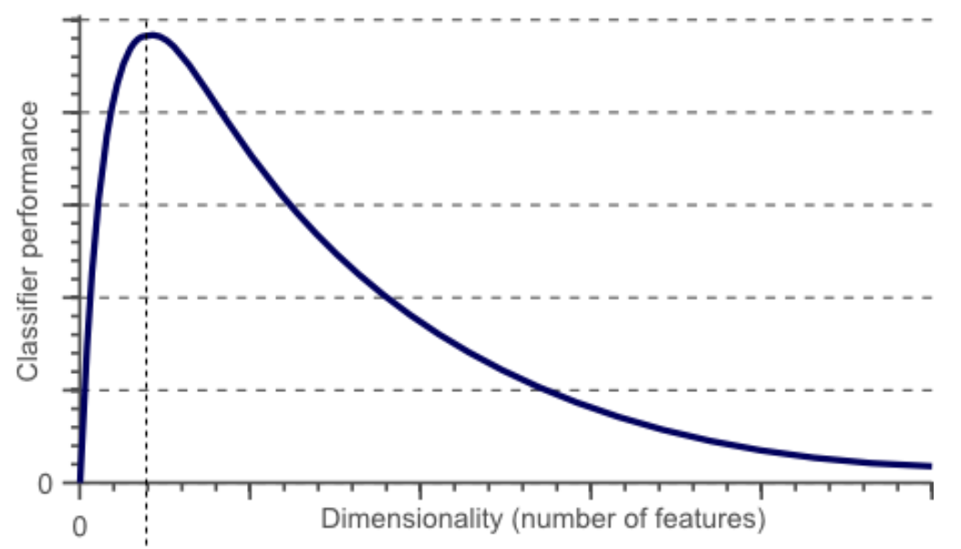
假設 data samples 為 N. Feature dimension 為 d.
-
一開始 feature dimension (d) 很小,無法有效的分類。如下圖 d = 0 附近。
-
(Bless of dimensionality) 增加 feature dimension (d),此時可以利用高維線性分類器 (對應低維的非線性分類器) 得到比較好的性能。如下圖的峰值位置。具體峰值對應的 d 和 : N,分類類別數,以及 data 的分佈有關。
-
(Curse of dimensionality) 再增加 feature dimension,則會有每個 feature dimension 的 data sparsity 的問題。高維的分類器雖然更容易分類,但會造成 overfit,導致分類器性能變差。如下圖峰值右邊性能掉落部分。這就是一種 curse of dimension.
https://www.visiondummy.com/2014/04/curse-dimensionality-affect-classification/
Curse of dimensionality in dynamic programming (Curve: search space!): all equal distance to find the nearest neighbor

在高維空間,於超立方體的體積來說,超球體的體積就變得微不足道了。因此,在某種意義上,幾乎所有的高維空間都遠離其中心,或者從另一個角度來看,高維單元空間可以說是幾乎完全由超立方體的「邊角」所組成的,沒有「中部」,這對於理解卡方分布是很重要的直覺理解。 給定一個單一分布,由於其最小值和最大值與最小值相比收斂於0,因此,其最小值和最大值的距離變得不可辨別。
這通常被引證為距離函數在高維環境下失去其意義的例子。
Introduction
1958 Rosenblatt 提出一種 neural network 稱爲 perceptron 用於分類幾何形狀 (也就是分割空間)。Perceptron 非常簡單如下。但被誇大 perceptron 可以用於 walk, talk, see, write, reproduce 等問題。 \(f(\mathbf{x})= \begin{cases}1 & \text { if } \mathbf{w} \cdot \mathbf{x}+b>0 \\ 0 & \text { otherwise }\end{cases}\) 不過在 1969 Minsky and Papert 所寫的書 “Perceptrons” 證明 (1-layer) perceptron 可以用於分類 linear separable 問題,但無法分類非 linear separable 的問題,最簡單的例子就是 XOR, 稱爲 Perceptron affair. 當時這件事打臉很大,變成所謂的第一次 AI hype.
解決 linear separable 問題很簡單,就是用兩層或多層的 perception. Cybenko (1989) 和 Hornik (1991) 證明使用兩層或多層 neural network 也可以生成密集類的功能,從而可以將任何連續函數近似為任何所需的精度-這種特性被稱為通用近似 (Universal Approximation)。但他們只給出存在性的證明,並沒有告訴如何找出這個 neural network nodes and weights. 也就是在早期 neural network 研究 learning algorithm 是一個 big challenge. 、
Rosenblatt 提出一個 learning algorithm 針對 1-layer perceptron. 另外 researchers 也有一些針對特定網絡的 learning algorithm.
Multi-layer Perceptron Learning - Back-propagation
再來就是 learning algorithm 的突破,backpropagation, 就是利用 loss function 計算 gradient of weights 並用 gradient descent-based optimzation technique to train neural network. 這也是 Hinton 的主要貢獻之一。
Curse of Dimensionality
Multi-layer neural network 雖然可以達成 universal approximation, 但沒有告訴我們要多大的網絡。一個質樸的想法就是用一個很大很深的神經網絡來近似任何函數。這會遇到另一個問題:curse of dimensionality, 或稱爲組合爆炸。注意 curve of dimensionality 和 overfitting 是完全不同的概念。
Curse 說明 1:Classifier (分類器),只有直覺,沒有數學
-
假設 data samples 為 N. Feature dimension 為 d.
-
一開始 feature dimension (d) 很小,無法有效的分類。如下圖 d = 0 附近。
-
增加 feature dimension (d),此時可以利用高維線性分類器 (對應低維的非線性分類器) 得到比較好的性能。如下圖的峰值位置。具體峰值對應的 d 和 : N,分類類別數,以及 data 的分佈有關。
-
再增加 feature dimension,則會有每個 feature dimension 的 data sparsity 的問題。高維的分類器雖然更容易分類,但會造成 overfit,導致分類器性能變差。如下圖峰值右邊性能掉落部分。這就是一種 curse of dimension.
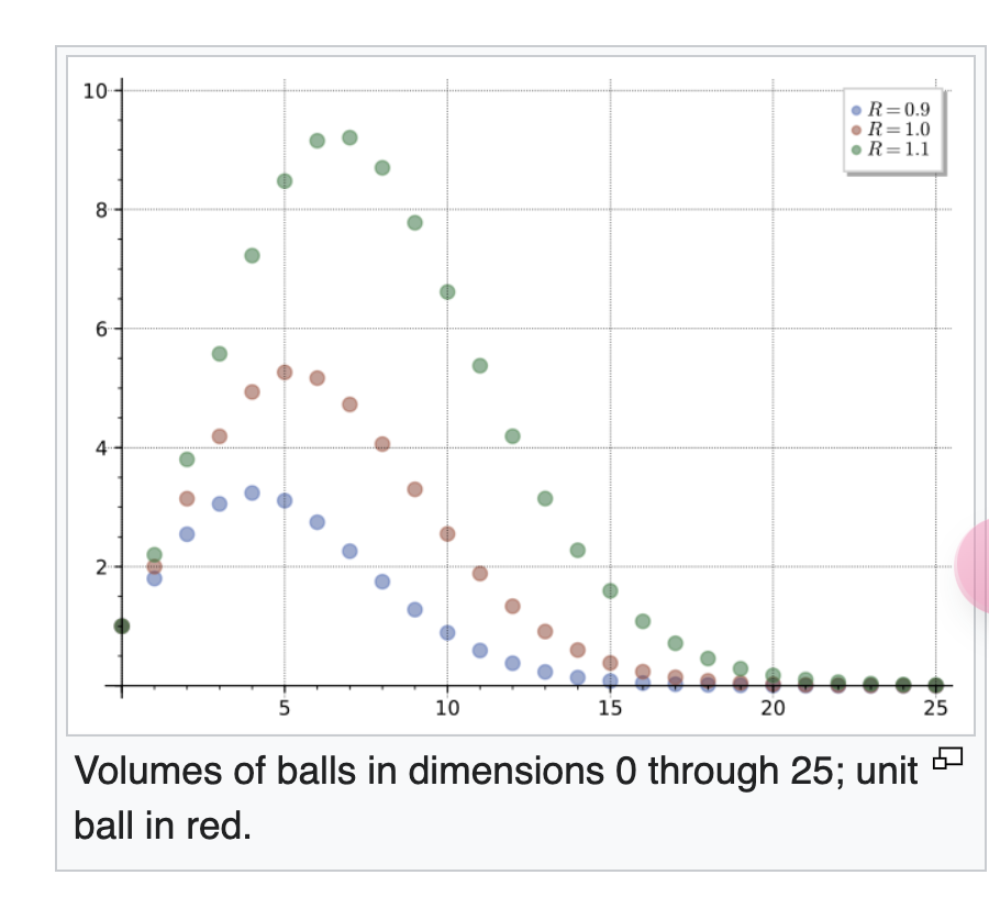
上圖是如何產生的?和 k dimension 的立體球的體積非常像!
Wiki: Volume of an n-ball. 這是巧合嗎?
以下是可能的猜測
什麽是一個有效的分類器?
-
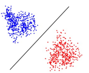
下圖是一個直覺的例子。就是同一類 data of the same feature 聚集在一起,但不同類 data (with different features) 有一定的距離。這裏我們假設有顔色作爲分別。但 in general 必須考慮 unsupervised learning, 也就是 data 沒有顔色,完全靠 clustering 來分類。因此 data 的數量要足夠才能像 cluster.
-
什麼是 data of the same feature? 我們可以用單位球 (unit sphere) 代表 feature space
- d=1, $2R$
- d=2, $\pi R^2$;
- d = 3, $\frac{4}{3} \pi R^3$;
- 當 d 越來越大如上上圖。先變大再變小。
- 下一個問題是 space between two clusters, 用正立方體代表:
-
d=1, $r$;
-
d=2, $r^2$;
-
d=3. $r^3$;
-
d dimension, $r^d$
-
-
如果 $r/2 > R$, e.g. $r = 2, R=1$
-
d=1, data 完全分離,也就是 100%
-
d=2, d=3, … 也是完全分離
-
似乎增加 feature dimension k 只是讓 data sparsity,而造成 overfit 性能下降。
-
-
如果 $r > R$, e.g. $r=1, R=1$
-
d=1, data 無法完全分離
-
增加 k 會讓 mixed data 更容易分離,性能變好。如上圖紅點。
-
再增加 feature dimension k 只是讓 data sparsity,而造成 overfit 性能下降。
-
-
如果讓 $R=0.9$,代表 feature 更集中,因此 feature dimension k 的 peak 值左移。
-
如果讓 $R=1.1$,代表 feature 更散開,因此 feature dimension k 的 peak 值右移。
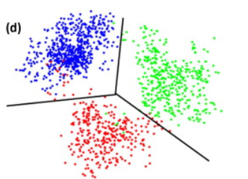
- 以上是二元分類。如果是多元分類,可以推導更多?
Curse 說明 2:球對立方體比例,沒有直覺,只有數學
一個常用來說明 curse of dimension 的 metric 是 n 維的球體佔 n 維空間 (就是 n 維立方體) 的比例,如下圖。
- d = 1,距離為 1 的 ”1 維球“,佔據 100% 的長度 1 的 “1 維空間”
- d = 2,距離為 1 的 ”2 維球“, $\int_0^r\int_0^{2\pi}r dr d\theta = \pi r^2$,佔據長度 1 的 “2 維空間” $\pi/4= 78.5$%
- d = 3,距離為 1 的 ”3 維球“,$\frac{4}{3}\pi r^3$,佔據長度 1 的 “3 維空間” $\frac{4}{3}\pi/8= \frac{\pi}{6} = 52.3$%

-
D = n,“n 維球“ 的體積是 (r=1) 如下式。
\[S_{n-1}=\frac{2 \pi^{n / 2}}{\Gamma\left(\frac{n}{2}\right)}, \quad V_n=\frac{\pi^{n / 2}}{\Gamma\left(\frac{n}{2}+1\right)}\] -
$\Gamma(\cdot)$ 是 gamma function。
- 如果上式 $n$ 是偶數,可以用 gamma function 正整數公式: $\Gamma(k) = (k-1)!$.
- 如果上式 $n$ 是奇數,可以用 gamma function 半正整數公式:
帶入上面 gamma function 定義: \(\begin{aligned} & \Gamma\left(\frac{1}{2}\right) = \sqrt{\pi} \approx 1.772, \quad & \Gamma\left(\frac{2}{2}\right) = 0! = 1, \quad & \Gamma\left(\frac{3}{2}\right) = \frac{1}{2} \sqrt{\pi} \approx 0.886, \quad & \Gamma\left(\frac{4}{2}\right) = 1! = 1 \\ & \Gamma\left(\frac{5}{2}\right) = \frac{3}{4} \sqrt{\pi} \approx 1.329, \quad & \Gamma\left(\frac{6}{2}\right) = 2! = 2, \quad & \Gamma\left(\frac{7}{2}\right) = \frac{15}{8} \sqrt{\pi} \approx 3.323, \quad & \Gamma\left(\frac{8}{2}\right) = 3! = 6 \\ \end{aligned}\)
帶入計算表面積和體積的公式:
-
n = 2, $S_1 = 2 \pi$ (周長);$V_2 = \pi$ (2D 圓面積)
-
n = 3, $S_2 = 2 \pi^{3/2}/\frac{\pi^{1/2}}{2} = 4\pi$ (2D 球面積);$V_3 = \pi^{3/2}/{4!/(4^2 2!) \sqrt{\pi}}= 4^2 2! \pi/4! = 16\cdot 2 \pi/24 = 4\pi/3$ (3D 球體積)
-
n = 4, $S_3 = 2 \pi^2/1! = 2\pi^2$ (3D 球面積);$V_4 = \pi^{2}/2! = \pi^2/2$ (4D 球體積)
在 n 維度中,單位球體的體積 $ V_n $ 可以與 n 維度中單位立方體的體積進行比較。n 維度中單位立方體的體積為 1。但此處是對比半徑為 1 的“單位球體”的體積。“單位立方體體積” 也要修正成 $2^n$。要了解 n 維度單位球體占單位立方體的比例,我們需要考慮 n 維度單位球體的體積。
n 維度單位球體 (半徑為 1) 的體積
\[V_n = \frac{\pi^{n/2}}{\Gamma\left(\frac{n}{2} + 1\right)}\]-
$ n = 1 $(從 -1 到 1 的線段):$V_1 = 2 $
-
$ n = 2 $ (單位圓): $V_2 = \pi$
-
$ n = 3 $ (三維空間中的單位球體):$ V_3 = \frac{4}{3}\pi $
-
$ n = 4 $ (四維空間中的單位球體):$ V_4 = \frac{1}{2}\pi^2 $
n 維度單位立方體 (邊長為 2) 的體積 = $2^n$
單位球體公式的近似
使用斯特林公式來近似伽馬函數,$\Gamma(x+1) = x! \approx \sqrt{2\pi x} \left(\frac{x}{e}\right)^x$,對於大的 $ n $:
$ \Gamma\left(\frac{n}{2} + 1\right) \approx \sqrt{2\pi \left(\frac{n}{2} \right)} \left(\frac{n/2}{e}\right)^{\frac{n}{2}} = \sqrt{\pi n} \left(\frac{n/2}{e}\right)^{\frac{n}{2}} $
因此:
\[V_n \approx \frac{\pi^{n/2}}{\sqrt{\pi n} \left(\frac{n/2}{e}\right)^{\frac{n}{2} }} = \left(\frac{2\pi e}{n}\right)^{n/2} \frac{1}{\sqrt{n\pi}}\]簡化這個表達式可以讓我們了解體積的行為。注意到 $ V_n $ 隨著 $ n $ 的增長迅速減少,因為項 $\left(\frac{n}{2} + 1\right)^{n/2}$ 的增長速度遠快於 $\pi^{n/2}$。
相對於單位立方體的比例
考慮到 n 維度中單位立方體的體積始終為 1,但考慮此處是對比半徑為 1 的“單位球體”的體積。“單位立方體體積” 也要修正成 $2^n$。
對於大的 $ n $:
\[\text{Ratio} \approx \left(\frac{2\pi e}{n}\right)^{n/2} \frac{1}{\sqrt{n\pi}} / 2^n = \left(\frac{\pi e}{2n}\right)^{n/2} \frac{1}{\sqrt{n\pi}} = \left(\frac{2.067}{\sqrt{n}}\right)^n \frac{1}{\sqrt{n\pi}} = 0.273 \left(\frac{2.067}{\sqrt{n}}\right)^{n+1}\]這個表達式顯示了隨著 $ n $ 的增長,單位球體相對於單位立方體的體積迅速減少。對於大的 $ n $,這個比例趨近於零,這意味著 n 維度單位球體在 n 維度單位立方體中占據的體積可以忽略不計。這是 curse of dimension 的一種解釋。
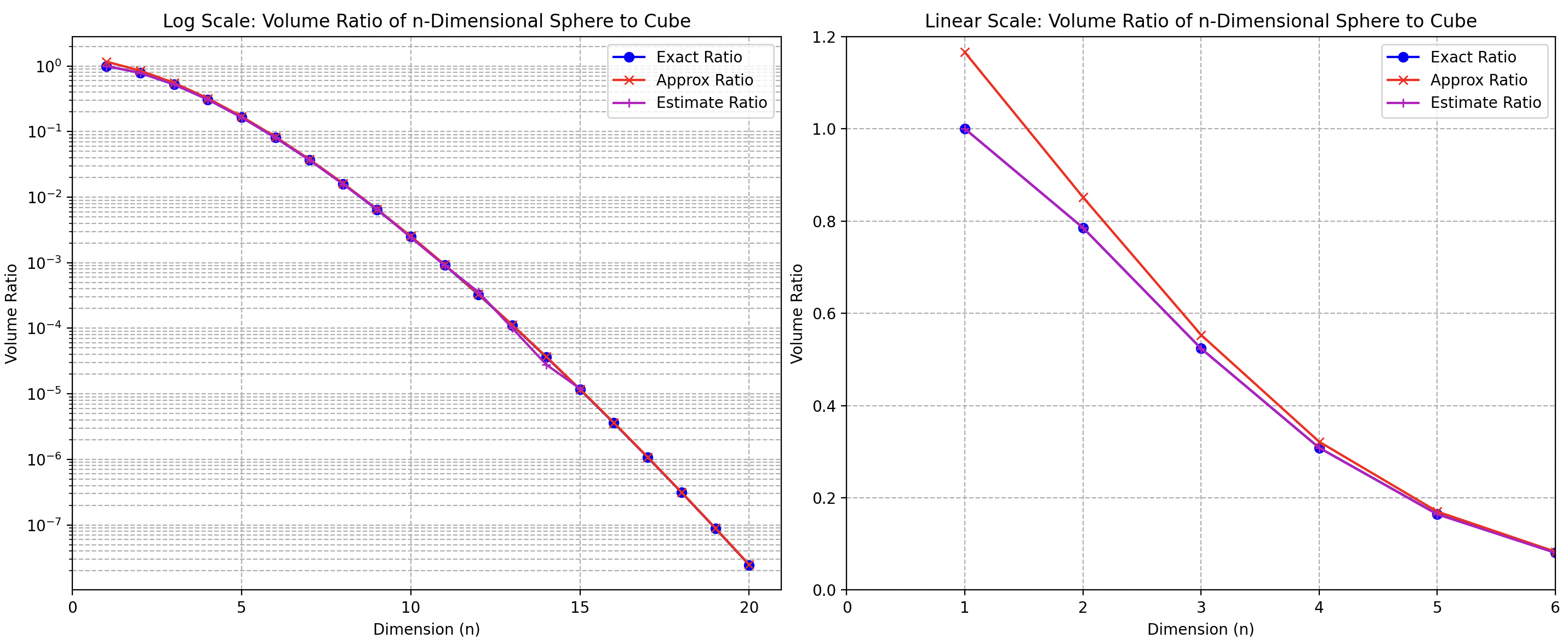
下圖包含三個方法計算 n 維 sphere to cube ratio:
- 第一個方法 (exact): 直接用計算 $\Gamma(\cdot)$。n = 1 是 100%,n = 2 是 78.5%,n = 3 是 52.3%。
- 第二個方法 (estimate): 使用統計取樣的方法計算。產生 n 維的 (-1, 1) 隨機變數 $(d_1, d_2, …, d_n)$,統計 $\sqrt{\Sigma_{k=1}^n {d_k^2}} <1$ 的比例。很明顯比例會隨著 n 變大而變小。
- 第一和第二種方法得到的結果基本一致,如下圖。但是在 n > 15,需要大量的樣本,並不容易產生。同樣 gamma function 在 n > 15 也不好計算。因此我們採用第三種方法。
- 第三種方法是用斯特林近似 (approximate)。如下圖紅線,在 n 足夠大和第一和第二方法一致。但在 n < 4 的誤差比較大。
Blessing of Dimensionality
(Physics) Statistics Mechanics –> Thermodynamic
(Machine Learning) Linearly separable

(Information Theory or Physics). AEP and Typical Set
Yes, the Asymptotic Equipartition Property (AEP) is related to high dimensionality, particularly in the context of information theory and statistics.
Asymptotic Equipartition Property (AEP)
The AEP states that for a large number of independent and identically distributed (i.i.d.) random variables drawn from a certain probability distribution, the sequences of outcomes will fall into a typical set where the probability of each sequence is approximately equal. This property is crucial in the field of information theory, where it underlies the concept of entropy and data compression.
Relationship to High Dimensionality
In high-dimensional spaces, the effects of the AEP become more pronounced. Here’s why:
-
Concentration of Measure: In high dimensions, the measure (or probability) tends to concentrate in certain regions of the space. For example, most of the volume of a high-dimensional sphere is concentrated near its surface. Similarly, the probability of sequences of outcomes will concentrate in a typical set as the dimension (or the number of observations) increases. This is a manifestation of the AEP.
-
Typical Sets: As dimensionality increases, the typical set (the set of sequences that have high probability) becomes a more precise representation of the source distribution. In other words, as the number of observations grows, almost all sequences will have a probability close to ( 2^{-nH(X)} ), where ( H(X) ) is the entropy of the source, and ( n ) is the number of observations. This indicates a strong relationship between high dimensionality and the AEP.
-
Data Compression: In high dimensions, the AEP ensures that data can be compressed efficiently. The typical set contains almost all the probability mass, meaning that one can encode the data using fewer bits per symbol on average, closely approaching the entropy rate ( H(X) ). This is particularly useful in high-dimensional data, such as images or long sequences of text.
Example in High Dimensions
Consider a high-dimensional vector where each component is an i.i.d. random variable following a specific distribution. According to the AEP, as the dimensionality increases, almost all vectors will have their empirical distributions close to the theoretical distribution of the random variable. This property is fundamental in statistical learning and high-dimensional data analysis.
Conclusion
The AEP is deeply connected to high dimensionality. As the number of dimensions (or the length of the sequence) increases, the observations tend to exhibit properties predicted by the AEP more strongly. This relationship is a cornerstone in information theory, enabling efficient data representation and compression in high-dimensional settings.
(Machine Learning) Data Compression (because of data concentration), GPTVQ

(Random) Sampling
作者:文兄 链接:https://www.zhihu.com/question/27836140/answer/141096216 来源:知乎 著作权归作者所有。商业转载请联系作者获得授权,非商业转载请注明出处。
维数增多主要会带来的高维空间数据稀疏化问题。简单地说:
- p=1,则单位球(简化为正值的情况)变为一条[0,1]之间的直线。如果我们有N个点,则在均匀分布的情况下,两点之间的距离为1/N。其实平均分布和完全随机分布的两两点之间平均距离这个概念大致是等价的,大家可稍微想象一下这个过程。
- p=2,单位球则是边长为1的正方形,如果还是只有N个点 ,则两点之间的平均距离为$\sqrt{\frac{1}{N}}$。换言之,如果我们还想维持两点之间平均距离为1/N,那么则需 $N^2$ 个点。重點是可以把這個問題轉換成 2 維球體佔正方形的問題。
- 以此类题,在 p 維空間,N个点两两之间的平均距离为 $N^{-\frac{1}{p}}$,或者需要 $N^p$ 个点来维持 1/N 的平均距离。
由此可见,高维空间使得数据变得更加稀疏。这里有一个重要的定理:N个点在p维单位球内随机分布,则随着p的增大,这些点会越来越远离单位球的中心,转而往外缘分散。这个定理源于各点距单位球中心距离的中间值计算公式:
\[d(p,N)=(1-\frac{1}{2}^{\frac{1}{N}})^\frac{1}{p}\]当p→∞时,d(p,N)→1。
很显然,当N变大时,这个距离趋近于0。直观的理解就是,想象我们有一堆气体分子,p变大使得空间变大,所以这些分子开始远离彼此;而N变大意味着有更多气体分子进来,所以两两之间难免更挤一些。
总之,当维数增大时,空间数据会变得更稀疏,这将导致bias和variance的增加,最后影响模型的预测效果。下图以KNN算法为例:
A good article:
https://www.visiondummy.com/2014/04/curse-dimensionality-affect-classification/
Two important points of DL
- Feature learning
- Back prop.
Curve of dimensionality 造成的後果
- 神經網路不是越大越好,因為 dimensionality 是 n1 x n2 x n3 …基本變成 diaster 除非
- 更多的 data : cost
- regularization
- 對稱性? CNN translation invariance/equivariance and share weights, not use Fully connected layer
- Otherwise overfitting
維度的詛咒
維度的詛咒指的是在高維空間中分析和組織數據時出現的各種現象。隨著維度數量的增加,這些問題使得某些任務變得越來越困難。以下是一些關鍵方面:
- 體積指數增長:
- 在高維空間中,空間的體積隨著維度數量呈指數增長。這意味著填充或表示空間所需的數據量變得非常龐大。
- 數據稀疏性:
- 隨著維度數量的增加,數據點變得稀疏。這種稀疏性使得難以找到有意義的模式、聚類或關係。
- 距離度量:
- 在高維空間中,任何兩點之間的距離幾乎變得均勻。傳統的距離度量(如歐幾里得距離)失去了區分能力,難以區分點之間的差異。
- 過度擬合:
- 高維數據會導致機器學習模型過度擬合。模型可能會捕捉到噪聲而不是潛在的模式,因為特徵數量相對於觀測數量過多。
- 計算複雜度:
- 算法的計算成本通常隨著維度數量顯著增加。優化、最近鄰搜索和函數逼近等任務變得更加計算密集。
維度的祝福
維度的祝福指的是高維空間所帶來的優勢和機會,特別是在機器學習和數據分析的背景下。以下是一些積極方面:
- 特徵豐富性:
- 高維空間允許表示更複雜的數據結構。更多的特徵可以捕捉到更多關於潛在數據生成過程的信息。
- 線性可分數據:
- 在高維空間中,數據點更可能是線性可分的。這可以使分類任務變得更容易,對於支持向量機(SVM)等算法有利。
- 稀疏表示:
- 高維空間可以導致數據的稀疏表示,這在壓縮感知和稀疏編碼等領域中是有用的。稀疏表示可以使數據存儲和處理更加高效。
- 維度縮減:
- 主成分分析(PCA)和t-SNE等技術利用高維空間找到保留數據主要特徵的低維表示。這些技術可以簡化數據分析和可視化。
- 模型的高容量:
- 在高維空間中,模型能夠有更高的容量來捕捉數據中的複雜模式和關係。這對於圖像和語音識別等複雜任務是有利的。
- 隨機投影:
- 隨機投影技術可以在保留距離和結構的同時降低數據的維度。這在簡化高維數據以便實際使用方面特別有用。
Dimension is Curse or Bless?
| 方面 | 維度的詛咒 | 維度的祝福 |
|---|---|---|
| 體積指數增長 | 空間體積指數增長,需要大量數據 | - |
| 數據稀疏性 | 數據點變得稀疏,使得模式識別變得困難 | - |
| 距離度量 | 距離變得幾乎均勻,度量失去效用 | - |
| 過度擬合 | 特徵數量過多導致模型過度擬合 | - |
| 計算複雜度 | 算法計算成本顯著增加 | - |
| 特徵豐富性 | - | 允許表示複雜結構 |
| 線性可分數據 | - | 更容易分類,線性可分性增強 |
| 稀疏表示 | - | 稀疏域中的高效數據存儲和處理 |
| 維度縮減 | - | 利用高維空間技術找到低維表示,簡化數據分析和可視化 |
| 模型的高容量 | - | 模型能夠捕捉數據中的複雜模式 |
| 隨機投影 | - | 在保留結構的同時簡化數據 |
總結來說,儘管高維空間帶來了重大挑戰,但它們也提供了獨特的機會和優勢,可以在數據分析和機器學習的各個領域中加以利用。
Appendix
Code example
1 | |
Reference
https://www.visiondummy.com/2014/04/curse-dimensionality-affect-classification/