Approach 1: From Hilbert ?? question
公理化機率和物理 (量子力學)
What? like digital twin, a parallel world indep. of real world.
Answer: by Komologov axiom
Von Neunman also axiomize quantum mechanics
Approach 2: From Application aspect
Experimentalist (frequencist) to Baysianist
Bayes formula : … The history of Bayes
概率的兩種方法:公理化和應用
概率論是一個數學分支,專門研究隨機現象的分析。其發展主要沿著兩條主線進行:概率的公理化和基於應用的解釋,包括貝葉斯和頻率主義的視角。這兩種方法為理解和應用概率提供了不同的框架,從抽象的數學理論到實際的實驗和決策。
方法一:概率的公理化
希爾伯特的第六問題
1900年,David Hilbert在國際數學家大會上提出了23個未解決的問題。其中,希爾伯特的第六問題要求對物理學進行公理化,特別是概率論的基本方面。這一挑戰旨在建立一個嚴格的數學框架來描述概率,類似於幾何學的公理。
Kolmogorov的公理
1933年,Andrey Kolmogorov制定了一套公理,奠定了現代概率論的基礎。這些公理被稱為Kolmogorov的公理,包括:
- 非負性:對於任何事件 $ A $,其概率 $ P(A) \geq 0 $。
- 規範化:整個樣本空間 $ S $ 的概率為1,即 $ P(S) = 1 $。
- 可加性:對於任何兩個互斥事件 $ A $ 和 $ B $,它們的聯合概率是其個別概率之和,即 $ P(A \cup B) = P(A) + P(B) $。
這些公理提供了一個一致且完整的框架來計算概率,並成為概率論的基石。
Von Neumann的量子力學公理化
在物理學領域,特別是量子力學中,John von Neumann擴展了公理化的方法。他引入了一個基於Hilbert空間的嚴格數學公式化,這是一種配有內積的抽象向量空間。Von Neumann的工作形式化了量子力學的概率性質,為理解量子層面的現象提供了堅實的基礎。
方法二:基於應用的解釋
頻率主義解釋
頻率主義的概率解釋,源於Ronald Fisher和Jerzy Neyman的工作,將概率視為事件的長期相對頻率。在這個框架下,概率被解釋為在重複試驗中觀察到的相對頻率的極限。例如,投擲硬幣出現正面的概率被理解為在大量投擲中觀察到正面的比例。
頻率主義方法強調使用實驗數據來估計概率和進行推斷。這種方法廣泛用於假設檢驗,其中計算在零假設下觀察到檢驗統計量的概率,以確定是否拒絕零假設。
貝葉斯解釋
貝葉斯方法,以Thomas Bayes牧師命名,將先驗知識或信念納入概率評估過程。貝葉斯定理是一個在此方法中的基本結果,允許基於新證據更新概率:
| $P(A | B) = \frac{P(B | A) \cdot P(A)}{P(B)}$ |
其中:
-
$ P(A B) $ 是在給定 $ B $ 的條件下 $ A $ 的後驗概率。 -
$ P(B A) $ 是在 $ A $ 發生的條件下 $ B $ 的似然。 - $ P(A) $ 是 $ A $ 的先驗概率。
- $ P(B) $ 是 $ B $ 的邊際概率。
貝葉斯方法提供了一個靈活的框架,用於在新數據可用時更新信念。這種方法在機器學習等領域特別有用,因為先驗知識可以顯著提高模型性能。
貝葉斯定理的歷史
貝葉斯定理首次出現在Thomas Bayes於1763年死後發表的一篇文章中,題為“解決機率學中問題的一篇論文”。這篇文章由Richard Price編輯並發表。雖然貝葉斯的工作為後來的貝葉斯概率奠定了基礎,但直到20世紀才獲得廣泛認可。Pierre-Simon Laplace進一步發展並推廣了這一定理,將其應用於天體力學和其他科學問題。
Edwin Jaynes是概率論和信息理論的重要貢獻者之一,他的思想對貝葉斯統計學有著深遠的影響。Jaynes主張,貝葉斯方法不僅是一種數學工具,而是一種更普遍的推理方式,可以應用於任何形式的不確定性下的推斷和決策。他強調了將先驗知識結合到概率推斷中的重要性,並提出了最大熵原理來解釋如何選擇最合適的概率分佈。
Jaynes的觀點推動了貝葉斯方法的應用範圍擴展,並對許多領域,包括物理學、工程學和社會科學,產生了深遠的影響。他的工作促使人們重新思考概率和統計推斷的基礎,並將貝葉斯方法視為一種更自然和普遍適用的推理方式,超越了傳統頻率主義的限制。
結論
公理化和基於應用的概率解釋提供了互補的視角。Kolmogorov的公理提供了一個嚴格的數學基礎,確保了概率推理的一致性和連貫性。而頻率主義和貝葉斯方法則提供了實際應用概率的框架,從實驗分析到不確定性下的決策。理解這兩種方法增強了我們駕馭和解釋世界中固有隨機性的能力。
Machine learning 就是一個 deterministic 和 probabilistic 擺盪和交織的過程。
(Input) dataset 一般是 deterministic.
傳統的 machine learning technique, e.g. linear regression, SVM, decision tree, etc. 也很多是 deterministic math.
但是 ML 背後的 modeling, 邏輯,和解釋卻可以用 probabilistic 統一解釋。例如 logistic regression, 甚至 neural network 的分類網路卻可以有 probability 的詮釋。
最後一類從頭到尾都是 probabilistic. 例如 bayesian inference, variational autoencoder.
假設我們都先限制在 training; all data; mini-batch (some randomness) or 1-point. Inference 都可以假設是 1-point.
| Input | Model | Output | Comment | |
|---|---|---|---|---|
| Linear regression | (D) all data | (D) linear function | (D) error | |
| Logistic regression | (D) all data | (D) logistic function | (P) probability distribution | distribution is a (D) function |
| Classification NN learning | (P) random minibatch data | (D) NN | (P) random gradient | Loss + SGD |
| Classification NN inference | (D) fixed 1-data | (D) NN | (P) probability distribution | |
| VAE training | (P) fixed 1-data | (D) NN | (P) random gradient | Loss + SGD |
| VAE encoder, training | (D) fixed 1-data | (D) NN | (P) parameter of distribution | parameter to RV |
| VAE decoder, generation | (P) random 1-sample from z | (D) NN | (P) random output variable | output sample |
| SVM | (D) dataset | (D) kernel function | (D) binary |
Some misc note
absolute deterministic: function, NN? (input/output), not parameter deterministic/probabilistic: random variable, distribution; ideal is random, but representation (function) is determinstic! probabilistic: sampling, MC
single data-point and collective data
我們分析什麼 input-model-output pattern 是合理的?
- D-D-D or P-P-P 顯然合理 (everything is deterministic or probabilistic)
- P-D-P or D-P-P 也合理 (probabilistic input or model 產生 probabilistic output)
- D-D-P 看起來奇怪需要解釋 (determinsitic input and model 產生 probabilistic output)
- D-P-D or P-P-D or P-D-D 似乎不 make sense (probabilistic input or model 產生 deterministic output)
Deterministic inside Probabilistic (D-D-P)
只看上表又太簡化。例如 input (D), model (D), 如何產生 output (P)?
我們更進一步分析 probabilistic: 包含 distribution 和 sampling.
- Distribution (function) 和 parameters 可以視為另一類 deterministic! 因為 distribution function 本身並非 random.
- 真正的 probabilistic 顯現在 randomness, 例如 Sampling 是 random, 也就是每次可能不同。
(D) Distribution and (P or Random) Sample 分布和採樣
以上的分析都是基於數學上的機率分布或是訊息論。實務上我們看不到摸不到機率分布或是 entropy/information,只有採樣 (sample) 和 Monte Carlo simulation.
我們先從機率分布 $p(x)$, $x$ 的期望值定義為: \(\mathbb{E}[x]=\int x p(x) d x\) 如果我們選擇 $x_o < x_1 < … < x_n$,數值積分變成 \(\mathbb{E}[x] \approx \sum_{i=1}^{n} x_{i} p\left(x_{i}\right)\left(x_{i}-x_{i-1}\right)\)
問題是我們可能根本不知道 $p(x_i)$,這就是有趣的部分:$p(x_i)(x_i - x_{i-1})$ 代表 $x_i$ 採樣出現的機率。也就是說其實我們不用做什麼事,只要“隨機採樣” $x_i$,就自帶機率部分。但是我們需要 normalize to total 採樣次數。 \(\mathbb{E}[x] \approx \frac{1}{n} \sum_{i=1}^{n} x_{i}, \quad x_{i} \sim p(x)\)
- 注意採樣的 $x_i$ 只要求隨機,並不要求有順序 $x_o < x_1 < … < x_n$.
- $p(x_i)$ 大的採樣機率自然大。採樣結果已經包含了 $p(x)$ 就不用再乘 $p(x)$, 也不用知道 $p(x)$ 到底是什麼。
- 可以推廣到一般的期望值 \(\mathbb{E}_{x \sim p(x)}[f(x)]=\int f(x) p(x) d x \approx \frac{1}{n} \sum_{i=1}^{n} f\left(x_{i}\right), \quad x_{i} \sim p(x)\)
這就是蒙地卡羅模擬的基礎。看起來簡單,實際上隨機採樣並不容易。 Gaussian distribution,uniform distribution 採樣很容易。但是一個複雜的 distribution 像是 image distribution 的採樣很困難。
Example 1: VAE Training
VAE loss function, 這是一個 expectation base on (D) distribution. 我們要 throw in (R) samples 才能 train encoder and decoder NN, i.e. $\theta, \phi$
\[\begin{aligned} \mathcal{L} &=\mathbb{E}_{x \sim \tilde{p}(x)}\left[\mathbb{E}_{z \sim p(z \mid x)}[-\ln q(x \mid z)]+\mathbb{E}_{z \sim p(z \mid x)}\left[\ln \frac{p(z \mid x)}{q(z)}\right]\right] \\ &=\mathbb{E}_{x \sim \tilde{p}(x)}\left[\mathbb{E}_{z \sim p(z \mid x)}[-\ln q(x \mid z)]+K L(p(z \mid x) \| q(z))\right] \end{aligned}\]Imagenet 的影像 sample 就不是隨機 sample, 有太多人為的選擇。 我們假設 for a fixed image $x_i$
\[l_{i}(\theta, \phi)=-E_{z \sim q_{\phi}\left(z | x_{i}\right)}\left[\log p_{\theta}(x_{i} | z)\right]+K L\left(q_{\phi}(z | x_{i}) \|\,p(z)\right)\]因為 $p(z)$ and $p_\theta(x’_i\mid z)$ 是由 Gaussian random variable 產生。基本符合“採樣”原則。$z$ 的 mean and variance 是從 $x_i$ 得到,一般不怎麼 random? 但是 training 大多使用 stochastic gradient descend (SGD), 算是比較 random? but the prior image set 依然不是 random, 也不一定是 $p(x)$ distribution. 我們假設 $x_i$ sample somehow follows $p(x)$ to make our life easier :)
\[\mathcal{L}=\mathbb{E}_{x \sim \tilde{p}(x)}[-\ln q(x \mid z)+K L(p(z \mid x) \| q(z))], \quad z \sim p(z \mid x)\]$x_i$ 得到 mean and variance. 第一個對 posterior expectation 可以用採樣取代。 KL 則可以用 close form!! which is $\mu^2 + \log \sigma$ (TBC)
因此可以採樣加上計算得到單一 $x_i$. 這就是 VAE 的 training 方式?
我們再看一些其他 training 例子。
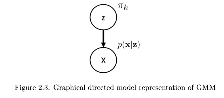
Fitting Latent Variable Models EM Algorithm
Expectation Maximization (EM) algorithm is widely used algorithm for fitting directed LVM models which aim is the same as in the case of maximum likelihood estimation - maximize data likelihood $p_{\theta}(x)$ for some model $p_{\theta}(x, z)$ of particular parametric family with parameters θ.
Having collected observable data points $\mathcal{D}={\mathbf{x}^{(1)}, \mathbf{x}^{(2)}, \cdots, \mathbf{x}^{(m)}}$ (where $m \ge 1$), we wish to maximize marginal log-likelihood of the data
\[\log \left[p_{\boldsymbol{\theta}}(\mathcal{D})\right]=\mathbb{E}_{\mathbf{x} \sim \mathcal{D}}\left[\log p_{\boldsymbol{\theta}}(\mathbf{x})\right]=\mathbb{E}_{\mathbf{x} \sim \mathcal{D}}\left[\mathbb{E}_{\mathbf{z} \sim p_{\boldsymbol{\theta}}(\mathbf{z} \mid \mathbf{x})}\left[\log p_{\boldsymbol{\theta}}(\mathbf{x}, \mathbf{z})\right]\right]\][@poczosCllusteringEM2015]
Example 2: Given Input 經過 Deterministic NN 轉成 Probabilistic Conditional Distribution
[@kingmaIntroductionVariational2019]
一般的 differentiable feed-forward neural networks are a particularly flexible and computationally scalable type of function approximator.
A particularly interesting application is probabilistic models, i.e. the use of neural networks for probability density functions (PDFs) or probability mass functions (PMFs) in probabilistic models (how?). Probabilistic models based on neural networks are computationally scalable since they allow for stochastic gradient-based optimization.
We will denote a deep NN as a vector function: NeuraNet(.). In case of neural entwork based image classifcation, for example, nerual networks parameterize a categorical distrbution $p_{\theta}(y\mid \mathbf{x})$ over a class label $y$, conditioned on an image $\mathbf{x}$. ??? y is a single label or distribution?
\[\begin{aligned} \mathbf{p} &=\operatorname{NeuralNet}_{\boldsymbol{\theta}}(\mathbf{x}) \\ p_{\boldsymbol{\theta}}(y \mid \mathbf{x}) &=\text { Categorical }(y ; \mathbf{p}) \end{aligned}\]where the last operation of NeuralNet(.) is typical a softmax() function! such that $\Sigma_i p_i = 1$
這是很有趣的觀點。 $\mathbf{x}$ and $\mathbf{p}$ 都是 deterministic, 甚至 softmax function 都是 deterministic. 但我們賦予最後的 $y$ probabilistic distribution 涵義!基本上 NN 分類網路都是如此 (e.g. VGG, ResNet, MobileNet)。
例如 $\mathbf{x}$ 可能是一張狗照片, $\mathbf{p}$ 是 feature extraction of $\mathbf{x}$. 兩者都是 deterministic. 但最後 categorical function 直接把 $\mathbf{p}$ 賦予多值的 (deterministic) distribution, 例如狗的機率 $p_1 = 0.8,$ 貓的機率 $p_2 = 0.15,$ 其他的機率 $p_3 = 0.05.$ 這和我們一般想像的機率性 outcome, 同一個 $\mathbf{p}$ 有時 output 狗,有時 output 貓不同。
數學上這只是 vector to vector conversion, $\mathbf{p}$ 是 high dimension feature vector (e.g. 1024x1), $\mathbf{y} = [y_1, y_2, \cdots]$ 是 low dimension output vector (e.g. 3x1 or 10x1) summing to 1. 重點是這個 low dimension vector $\mathbf{y}$ 就是 conditional distribution! 也就是一個 sample $\mathbf{x}$ 就可以 output 一個 conditional distribution, 而不需要很多 $\mathbf{x}$ samples 產生 conditional distribution! 這很像量子力學中一個電子就可以產生 wave distribution, 有點違反直覺。
這似乎是把一個 random sample 轉換成一個 (deterministic) conditional distribution 的方式。不過是否是 general method, TBC.
Example 3: Multivariate Bernoulli data (3 產生 conditional distribution 的方法和 2 一樣)
一個簡單的例子說明 hand-waving 的 assertion for the DLVM.
Prior $p(z)$ 是簡單的 normal distribution. Neural network 把 random sample $z$ 轉換成 $\mathbf{p}$, 再來 $\mathbf{p}$ 直接變成 Bernoulli distribution! 就像例三的 softmax 一樣。
Likelihood $\log p(x\mid z)$ 因此也是簡單的 cross-entropy, i.e. maximum likelihood ~ minimum cross-entropy loss
\[\begin{aligned} p(\mathbf{z}) &=\mathcal{N}(\mathbf{z} ; 0, \mathbf{I}) \\ \mathbf{p} &=\text { DecoderNeuralNet }_{\boldsymbol{\theta}}(\mathbf{z}) \\ \log p(\mathbf{x} \mid \mathbf{z}) &=\sum_{j=1}^{D} \log p\left(x_{j} \mid \mathbf{z}\right)=\sum_{j=1}^{D} \log \operatorname{Bernoulli}\left(x_{j} ; p_{j}\right) \\ &=\sum_{j=1}^{D} x_{j} \log p_{j}+\left(1-x_{j}\right) \log \left(1-p_{j}\right) \end{aligned}\]where $\forall p_j \in \mathbf{p}: 0 \le p_j \le 1$
Joint distribution $p_{\boldsymbol{\theta}}(\mathbf{x}, \mathbf{z})=p_{\boldsymbol{\theta}}(\mathbf{z}) p_{\boldsymbol{\theta}}(\mathbf{x} \mid \mathbf{z})$ 就是把兩者乘積。雖然看起來 messy, 還夾著 neural network, 但理論上 straightforward, 甚至可以寫出 analytical form.
但反過來: posterior $p(z\mid x)$, marginal likelihood $p(x)$ 即使在這麼簡單的 network, 都是難啃的骨頭!
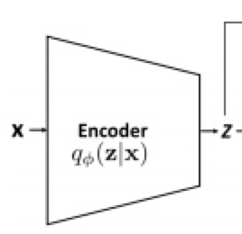
Example 4:Given Input 經過 Deterministic NN 轉成 Parameters of A Random Variable to Create Conditional Distribution (e.g. VAE encoder)
Example 2 and 3 NN 產生 conditional distribution 的方式只能用在 discrete distribution. 對於 continuous distribution, NN 無法產生無限長的 distribution! 例如 VAE 使用 Normal distribution 如下:
\[\begin{aligned} (\boldsymbol{\mu}, \log \boldsymbol{\sigma}) &=\text { EncoderNeuralNet }_{\boldsymbol{\phi}}(\mathbf{x}) \\ q_{\boldsymbol{\phi}}(\mathbf{z} \mid \mathbf{x}) &=\mathcal{N}(\mathbf{z} ; \boldsymbol{\mu}, \operatorname{diag}(\boldsymbol{\sigma})) \end{aligned}\]Neural network 產生 $\mu, \log \sigma$ for normal distribution. 雖然這解決 deterministic to probabilistic 問題。但聽起來還是有點魔幻寫實方式把 deterministic to probabilistic. 這是 VAE 的實際做法。
雖然的確產生 conditional distribtuion, 但似乎比直接產生 distribution 更不直觀!例如為什麼是 $\log \sigma$, 不是 $\sigma$ 或 $1/\sigma$ ? 另外只產生 $\mu, \log \sigma$ 兩個 parameters, 是否太簡化? 比起 softmax distribution 可能包含 10-100 parameters.
Before we can answer this question, let me quote below and move on to algorithm.
Typically, we use a single encoder neural network to perform posterior inference over all of the datapoints in our dataset. This can be contrasted to more traditional variational inference methods where the variational parameters are not shared, but instead separately and iteratively optimized per datapoint. The strategy used in VAEs of sharing variational parameters across datapoints is also called amortized variational inference (Gershman and Goodman, 2014). With amortized inference we can avoid a per-datapoint optimization loop, and leverage the efficiency of SGD.
Example 5: Decoder: How to explain $p(x\mid z)$ 的 conditional distribution?
https://towardsdatascience.com/understanding-variational-autoencoders-vaes-f70510919f73
Let’s now make the assumption that p(z) is a standard Gaussian distribution and that $p(x\mid z)$ is a Gaussian distribution whose mean is defined by a deterministic function f of the variable of z and whose covariance matrix has the form of a positive constant c that multiplies the identity matrix I. The function f is assumed to belong to a family of functions denoted F that is left unspecified for the moment and that will be chosen later. Thus, we have (不是很 make sense!)
\[\begin{aligned}(\boldsymbol{f(z)}) &=\text { DecoderNeuralNet }_{\boldsymbol{\theta}}(\mathbf{z}) \\p_{\boldsymbol{\theta}}(\mathbf{x} \mid \mathbf{z}) &=\mathcal{N}(\mathbf{x} ; \boldsymbol{f(z)}, c)\end{aligned}\] \[\begin{aligned} &p(z) \equiv \mathcal{N}(0, I) \\ &p(x \mid z) \equiv \mathcal{N}(f(z), c I) \quad f \in F \quad c>0 \end{aligned}\]What is $c$? 似乎只能 heuristically 解釋,沒有很 solid math fondation.
一個 random generator 不夠解釋 encoder and decoder? 那就兩個
我再想了一下,其實這可以視為 $z$ 的定義問題。我們借用 reparameterization trick 的 encoder formulation for $z$ 如下:
\[\begin{aligned}\boldsymbol{\epsilon} & \sim \mathcal{N}(0, \mathbf{I}) \$\boldsymbol{\mu}, \log \boldsymbol{\sigma}) &=\text { EncoderNeuralNet }_{\phi}(\mathbf{x}) \\\mathbf{z} &=\boldsymbol{\mu}+\boldsymbol{\sigma} \odot \boldsymbol{\epsilon}\end{aligned}\]我們可以分解 $\boldsymbol{\epsilon} = \boldsymbol{\epsilon}_1 + \boldsymbol{\epsilon}_2$ 都是 random variables.
\[\begin{aligned} \boldsymbol{\epsilon_1}, \boldsymbol{\epsilon_2} & \sim \mathcal{N}(0, \mathbf{I}/\sqrt{2}) \\ (\boldsymbol{\mu}, \log \boldsymbol{\sigma}) &=\text { EncoderNeuralNet }_{\phi}(\mathbf{x}) \\ \mathbf{z}' &=\boldsymbol{\mu}+\boldsymbol{\sigma} \odot \boldsymbol{\epsilon_1} \\ \boldsymbol{f(z')} &=\text { DecoderNeuralNet }_{\boldsymbol{\theta}}(\mathbf{z'}) \\ \mathbf{x}' = \boldsymbol{f(z')}+\boldsymbol{\delta} &=\text { DecoderNeuralNet }_{\boldsymbol{\theta}}(\mathbf{z}'+\boldsymbol{\sigma} \odot \boldsymbol{\epsilon}_2) \\ p_{\boldsymbol{\theta}}(\mathbf{x}' \mid \mathbf{z}') &=\mathcal{N}(\mathbf{x}' ; \boldsymbol{f(z')}, c) \end{aligned}\]where $c$ is the standard deviation of $\boldsymbol{\delta}$. 用 $z$’ 取代 $z$.
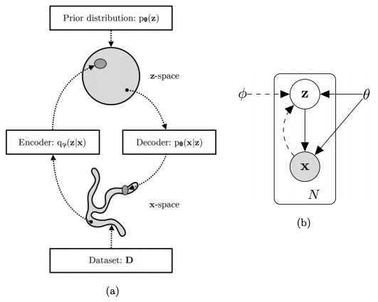
VAE Example
p(x): prior
p(z|x): likelihood
p(x|z): posterior
還是應該反過來?
$p(z)$: prior $p(x|z)$: likelihood, decoder $p(z|x)$: posterior, encoder
$I(X; Z) = H(X) - H(X\mid Z) \ge H(X) - R(X\mid Z)$ where $R(X\mid Z)$ denotes the expected reconstruction error of $X$ given the codes $Y$.
\[\begin{aligned} I(X; Z) &= D_{KL} (p_{(X,Z)} \| p_X p_Z) = E_X [D_{KL} (p_{(Z\mid X)} \| p_Z)] = H(X) - H(X\mid Z) \\ &= H(X) + \iint p(x, z) \log p(x\mid z) d x d z \\ &= H(X) + \int p(x) \left[ \int q(z \mid x) \log p(x\mid z) d z \right] d x \\ &= H(X) + \mathbb{E}_{x \sim p(x)}\left[\mathbb{E}_{z \sim q_{\phi}(z | x)}[\log p_{\theta}(x | z)]\right] \\ & \ge H(X) + \mathbb{E}_{x \sim \tilde{p}(x)}\left[\mathbb{E}_{z \sim q_{\phi}(z | x)}[\log p_{\theta}(x | z)]\right] \\ E_X [D_{KL} (p_{(Z|X)} \| p_Z)] &= H(X) + \mathbb{E}_{x \sim p(x)}\left[\mathbb{E}_{z \sim q_{\phi}(z | x)}[\log p_{\theta}(x | z)]\right] \end{aligned}\]or
\[\begin{aligned} H(X) = E_X [D_{KL} (p_{(Z|X)} \| p_Z)] - \mathbb{E}_{x \sim p(x)}\left[\mathbb{E}_{z \sim q_{\phi}(z | x)}[\log p_{\theta}(x | z)]\right] \end{aligned}\]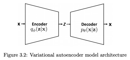
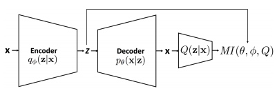
Variational Mutual Information
From $I(z; x) = H(z) - H(z\mid x)$
\[\begin{aligned} I(\mathbf{z} ; \mathbf{x})=& H(\mathbf{z})-H(\mathbf{z} \mid \mathbf{x}) \\ =& \mathbb{E}_{\mathbf{x} \sim p_{\theta}(\mathbf{x} \mid \mathbf{z})}\left[\mathbb{E}_{\mathbf{z} \sim q_{\phi}(\mathbf{z} \mid \mathbf{x})}[\log P(\mathbf{z} \mid \mathbf{x})]\right]+H(\mathbf{z}) \\ =& \mathbb{E}_{\mathbf{x} \sim p_{\theta}(\mathbf{x} \mid \mathbf{z})}\left[D_{K L}(P(\cdot \mid x) \| Q(\cdot \mid x))\right.\\ &\left.+\mathbb{E}_{\mathbf{z}^{\prime} \sim q_{\phi}(\mathbf{z} \mid \mathbf{x})}\left[\log Q\left(\mathbf{z}^{\prime} \mid \mathbf{x}\right)\right]\right]+H(\mathbf{z}) \\ \geq & \mathbb{E}_{\mathbf{x} \sim p_{\theta}(\mathbf{x} \mid \mathbf{z})}\left[\mathbb{E}_{\mathbf{z}^{\prime} \sim q_{\phi}(\mathbf{z} \mid \mathbf{x})}\left[\log Q\left(\mathbf{z}^{\prime} \mid \mathbf{x}\right)\right]\right]+H(\mathbf{z}) \end{aligned}\]where $Q$ is auxiliary distribution.
Graph Representation and EM Algorithm
這是 GNN 最簡單的例子。