Generative AI- Diffusion Lecture

Excellent lectures!!!!: https://www.youtube.com/watch?v=8mxCNMJ7dHM&list=PL0H3pMD88m8XPBlWoWGyal45MtnwKLSkQ

Main Reference

https://arxiv.org/pdf/1503.03585.pdf : original Stanford Diffusion paper: very good!

https://lilianweng.github.io/posts/2021-07-11-diffusion-models/ : good blog article including conditional diffusion

https://jalammar.github.io/illustrated-stable-diffusion/ by Jay Alammar, excellent and no math!

[@alammarIllustratedStable2022a] by Jay Alammar, excellent and no math!

[@alammarIllustratedStable2022] by Jay Alammar, excellent and no math!

Takeaways

1. Diffusion 使用的 chain rule 是 based on Markovian (所以和 Auto-Regressive 不同)
2. KL Divergence vs. W distance and their close form in Gaussian distribution
3. Mutual information: KL of P(x, y) // p(x) p(y)

爲什麽 AI 可以處理 ill-conditioned problem? 因爲有 underlying PDF!! 如果我們知道 PDF 或是可以 estimate PDF (或是用 data training 接近 underlying pdf), 我們就可以解決或是 optimize 很多 ill-conditioned problem!!

Key Assumptions/Observation of Image Space and Image Manifold

1. High dimension 基本 image space 是一個沙漠，絕大多數的地方都是沙。
2. Low dimension image manifold 沙漠中的綠洲. 所以我們只要知道 P(x), 基本可以完全得到所有 information. 這和通信完全不同！！！！ 因爲通信的 communication space 是 low dimension!! 所以一旦 signal and noise 混在一起就很難分離。但是 image space 是非常high dimensional.
3. What about audio space? LLM space? and other spaces?
4. 一個例子是 DC 信號或是極低頻信號，加上 gaussian noise 後，還是可以 estimate noise! 因爲 DC 信號是 low dimension (0), 但是 gaussian 信號是 very high dimensional.

Don’t do denoise in pixel space? but in latent space? 因爲在 latent space 對 noise 更高維？

Denoiser 是關鍵！MMSE denoise 就是 score function!

知道 $P(\bar{x})$ 就可以做所有 image processing and generation 和傳統的 DSP 完全不同。

1. 很多傳統 DSP 視為 ill-condition (e.g. super-resolution, deblur) 或是不可能 (e.g. image generation) 的問題。可以用 linear Inverse problem 描述。在知道 P(x), joint pdf or marginal pdf 後就變成可解的問題。如何得到 P(x)? 早期是靠猜。目前是靠 data training!
2. 其中 image generation 是傳統 DSP 完全無法解的問題！利用 P(x) 可以用來解！幾個方法：
   1. VAE: 利用 reconstruction loss + KL loss to train a generator.
   2. GAN
   3. Normalized Flow
   4. EBM (energy based model)
   5. Diffusion method!! -> randomly generate image then move to higher P(x), score-based 就是 diffusion
3. 實際上我們不是真正知道 P(x), 而是訓練一個 generator or sampler, $x_s = G_{\theta}(z_s)$, $x_s$ 的 distribution 符合 P(x)。
4. 如何從 generator G(z) 做其他的事，例如 linear inverse problem, SR, NR, compression…？

Exponential Family, Gibbs distribution is a Key,

![[Pasted image 20250122102634.png]]

Gibbs distribution: 似乎從 exponential family 得到靈感。轉換 P(x) to partition function and exponent!! 有點像 divide-and-conquer 但是利用 probability function 的特性 0 < P(x) < 1, $\rho(x)$ always positive

$P(x) = C \exp(-\rho(x))$

In the neural network $\theta$

$P(x) = \frac{1}{Z_{\theta}} \exp(-\rho_{\theta}(x))$

Diffusion Method Key Concept

利用 maximum likelihood on all image samples

$\max_{\theta} P(x_1) P(x_2)… P(x_n) = \max_{\theta} \Pi_k \frac{1}{Z^k_{\theta}} \exp(-\rho_{\theta}(x_k)) = \min_{\theta} { \log Z_{\theta} + \frac{1}{k}\Sigma_k \rho_{\theta}(x_k)}$

• 注意我們把 maximize P(x) 的問題轉換成 minimize $\rho_{\theta}(x_k)$
• 如果忽略 $Z_{\theta}$ 只是 minimize $\rho_{\theta}(x_k)$ 非常簡單
• 但重點是要考慮 $Z_{\theta}$, partition function, 問題變成複雜。各種方法就是爲了避免計算 $Z_{\theta}$

反向問題：如果有 $\rho_{\theta}(x)$, 如何生成 good quality image?

• start with any random x
• 找到 $\rho_{\theta}(x)$ 的 gradient on $x$, 然後做 gradient descent on $x$?

為什麼 image generation like diffusion 是 iterative? 因為這是 1st order optimization. 如果知道 image manifold, 是否可以 2nd order？ Or Flow method?

![[Pasted image 20250118235632.png]]

![[Pasted image 20250118235116.png]

![[Pasted image 20250119001855.png]]

![[Pasted image 20250119002252.png]]

![[Pasted image 20250119002622.png]]

![[Pasted image 20250119003906.png]]

![[Pasted image 20250119005034.png]]

![[Pasted image 20250119010327.png]]

![[Pasted image 20250119010436.png]]

Deep Learning for Computer Vision/Image

1. ImageNet: DL supervised learning for classification: discriminative problem
2. DL for regression: supervised learning discriminative problem
3. DL Variational AE: new sample generation based on existing samples via self-supervised learning
4. DL Diffusion: generation based on Markovian property

Generation P(x) 的 samples 並不等於有 P(x) 的 distribution!!!!
可以參考 [[2024-05-26-Math_Sampling]] ![[Pasted image 20250119121811.png]]

不過兩者是緊密相連。

1. 如果有 P(x), 可以用 random number generator 加上 inverse CDF, transformation, 或是 MCMC (Monte Carlo Markov Chian) 產生 samples, 這個過程稱爲 sampling. P(x) –> G 比較直覺容易。不過一般沒有這麽好的事，prior P(x).
   1. 如何利用 score function 產生 sample. 這是 MCMC sampling.
   2. 下一個問題是如何得到這個 score function?
2. 相反，如果有 G, 我們可以 generate 出很多 samples, 統計 mean, variance, … , and histogram 似乎可以近似一個 P(x). 只是沒有效率。
3. 同樣，如果有 G 而不是 P(x)

### Question1a: Given P(x), 如何產生 sample (也就是 sampler) 或是 generation model!

有很多方法可以產生 samples. 我們這裏從 MCMC 開始。利用 Langevin dynamics. 只要有 score function, 我們可以產生 emirical samples 符合 P(x)! 這只是方法之一，但是太慢。要用別的方法加速。

這是第一個 diffusion equation! Diffusion 是指 P(X(t)) over time.

![[Pasted image 20250125221658.png]] ![[Pasted image 20250125224405.png]] Don’t use Langevin for practicality because it takes 10,000 steps to converge. Only for theoretical analysis.

Question1b: 如何得到或是近似 score function?

簡單答案就是 denoiser! 正確的説法是 denoiser - original image = noise. 也就是 noise estimator!! 如何得到 denoiser, 使用 neural network!! 也就是說 Lengevin equation 中唯一的 learnable part 就是 denoiser, D! 但是這裡的 denoiser 非常簡單，只需要在一個固定而且很小的 noise (sigma=0.01) 的 denoiser. 代價就是非常久收斂！

Question 1c: 如何加速 Langevin equation?

簡單的答案是 “自污”! 壞事傳千里。Technical term: annealing, or annealing diffusion ![[Pasted image 20250125223926.png]]

It takes about 1000 steps to restore the image. ![[Pasted image 20250125224327.png]] 也就是說 Annealed Lengevin equation (AVD) 中唯一的 learnable part 就是 denoiser, D! AVD 的 denoiser 和前面的 denoiser 不同，必須在各種大小 noise 的 denoiser! 所以訓練會比較困難！

Question 1d: Use mixture of image and noise instead of additive noise!

![[Pasted image 20250125224818.png]] ![[Pasted image 20250125225037.png]] 也就是說 Annealed Lengevin equation (AVD) 中唯一的 learnable part 就是 denoiser, D! 這裡的 denoise 和 AVD 又不同！是在 image 和 noise 呈現 mixture 時的 denoise! AVD 的 denoiser 是固定 image, denoise 不同大小的 noiser. 這裡是 image 會變化。如果從 SNR 角度，兩者差不多。注意這裡的 denoiser 和後面 DDPM 非常像！

Question 1e: DDPM and 1f: DDIM

DDPM 的重點是 backward path 的 denoise 也是 Gaussian 當 step $\tau$ 很小，而且 iteration K 很大，基本就是 Gaussian noise. 一旦是 Gaussian, 就有 analytic form.

DDPM 也是 denoiser. 不過又是另一種 denoiser. 他不是 denoise 所有 noise 回到原來 image, 而是 denoise 一點 noise, 回到前一個 noisy image. 這樣比較好訓練？

Denoising Diffusion Probabilistic Models (DDPM) and Denoising Diffusion Implicit Models (DDIM) are both types of diffusion models used in generative AI, but they differ in their approach to the reverse process and sampling efficiency.

Similarities

1. Both DDPM and DDIM use the same forward process, gradually adding Gaussian noise to data over a series of timesteps[2].

2. They share the same training objective, allowing DDIM to use pre-trained DDPM models for inference[6].

3. Both models aim to learn the data distribution through forward and reverse diffusion processes[6].

Comparison between DDPM and DDIM in Perplexity

Differences

Reverse Process

• DDPM uses a probabilistic reverse process, learning to denoise data step-by-step[2].
• DDIM modifies the reverse process to make it deterministic, defining a fixed mapping between timesteps[2].

Sampling Efficiency

• DDIM allows for much faster sampling compared to DDPM, making it competitive with GANs in terms of generation speed[4].
• DDIM can generate samples in fewer steps, offering a trade-off between sample quality and computational efficiency[2].

Mathematical Formulation

• DDPM’s reverse process is Markovian, while DDIM introduces a non-Markovian forward process[1][2].
• DDIM sets the forward posterior variance to zero, allowing it to skip diffusion timesteps inside subsequences[6].

Performance

• DDIM can be 10 to 50 times faster than previous conditional diffusion methods while maintaining comparable quality[3].
• DDIM provides a family of generative models that can be chosen by selecting different non-Markovian diffusion processes[4].

In essence, DDPM focuses on probabilistic denoising, while DDIM introduces deterministic sampling for improved efficiency without sacrificing the model’s generative capabilities[2].

Citations: [1] https://arxiv.org/html/2402.13369v1 [2] https://aman.ai/primers/ai/diffusion-models/ [3] https://openreview.net/forum?id=8xStV6KJEr [4] https://strikingloo.github.io/wiki/ddim [5] https://www.tonyduan.com/diffusion/ddpm_vs_ddim.html [6] https://redstarhong.tistory.com/312 [7] https://sachinruk.github.io/blog/2024-02-11-DDPM-to-DDIM.html [8] https://www.reddit.com/r/StableDiffusion/comments/zgu6wd/can_anyone_explain_differences_between_sampling/

| | DDPM | DDIM | Note | | ——– | ——————————————— | ——————————————- | ——————————————- | | Forward | Force Markovian and additive Gassian | Non-Markovian, but additive Gaussian | share the same denoiser!! | | Backward | Approx. Gaussian and Markovian for small step | Force Markovian!! set to be deterministic! | DDIM is fast because deterministic backward | | | | | | Catch:

• Use DDPM 訓練一個 forward path denoiser, 同樣 denoiser 可以用在 DDIM
• 使用 DDIM 作為 inference, 因為比較快而且 image consistency.

另外還有 CM (Consistency Model) 也是用於加速, 比較如下：

Consistency Models (CM) and Denoising Diffusion Implicit Models (DDIM) are both advancements in generative AI that aim to improve the efficiency of diffusion models. Here’s a comparison of their key features:

Similarities

1. Both CM and DDIM are designed to accelerate the sampling process of diffusion models.

2. They both aim to produce high-quality samples more efficiently than traditional Denoising Diffusion Probabilistic Models (DDPMs).

3. CM and DDIM can be trained using pre-trained diffusion models[1][2].

Differences

Sampling Process

• DDIM modifies the reverse process of DDPMs to make it deterministic, allowing for faster sampling[2].
• CM aims to directly map noise to data in a single step or very few steps[8].

Flexibility

• DDIM allows for a trade-off between computation and sample quality by adjusting the number of sampling steps[2].
• CM supports both one-step generation and multi-step sampling, offering more flexibility in balancing speed and quality[8].

Training Objective

• DDIM uses the same training objective as DDPMs, making it compatible with pre-trained DDPM models[2].
• CM introduces a new training approach called Consistency Training (CT), which is more challenging but potentially more powerful[9].

Performance

• DDIM can produce samples 10 to 50 times faster than DDPMs in terms of wall-clock time[2].
• CM claims to achieve state-of-the-art results in one-step generation, with competitive performance even in just two sampling steps[8].

Additional Capabilities

• DDIM allows for semantically meaningful image interpolation in the latent space[5].
• CM supports zero-shot editing tasks like image inpainting and super-resolution without specific training[8].

In essence, while both CM and DDIM aim to improve the efficiency of diffusion models, CM represents a more radical departure from traditional diffusion model architecture, potentially offering even faster generation at the cost of more complex training.

Citations: [1] https://openaccess.thecvf.com/content/CVPR2024/papers/Xu_Inversion-Free_Image_Editing_with_Language-Guided_Diffusion_Models_CVPR_2024_paper.pdf [2] https://openreview.net/forum?id=St1giarCHLP [3] https://github.com/alexander-soare/consistency_policy [4] https://arxiv.org/html/2411.08954v1 [5] https://strikingloo.github.io/wiki/ddim [6] https://slazebni.cs.illinois.edu/spring24/lec13_diffusion_viraj.pdf [7] https://www.roboticsproceedings.org/rss20/p071.pdf [8] https://www.semanticscholar.org/paper/Consistency-Models-Song-Dhariwal/ac974291d7e3a152067382675524f3e3c2ded11b [9] https://arxiv.org/html/2403.06807v2

Question2: 如何從 G (diffusion) 得到 P(x)?

以 diffusion DDPM 和 DDIM 非常容易： P(x) ~ P(x1 |x0) P(x2 | x1) …

Question3: 如何從 G (diffusion) 做 super resolution, compression, etc.

Guided Diffusion

1. class guide
2. image guide
3. text guide

Class guide

利用 AVD as example, ![[Pasted image 20250125232312.png]]

Key 是找到新的 conditional score function, how?

• Guess 1: 只對 class = c 的 image 訓練 D_c denoiser? 不實際，需要太多 denoiser 而且 sample 太少。
• Guess 2: 需要加一個向 class = c 的力。How? 就是 classifer 的 back-propagation gradient! 但是這個 classifier 是一個可以 detect noisy image 的 classifer. 而且在
• ![[Pasted image 20250125233311.png]]

![[Pasted image 20250125234659.png]]

Question2: 如何從 P(x) samples 得到 distribution, 然後可以做 classification, denoise, super resolution? 如同在 LLM decoder, 如何用 LLM decoder 做 sentiment detection, 或是 spam detection? 可以直接用問的。或是利用最後一層做 fine-tune!

Nonlinear history of AI 三個 key events:

1. (Physics related) Iscing equation to Hpfield: use neuron and lowest energy to find the ground state.
2. (Some physics related) RBM: organized neurons, hidden unit, and introduce randomness, then back-prop
3. (No physics analog?) Variational autoencoder: stack RBM
4. (Physics related) diffusion!

	Ising 模型	Hopfield 神經網絡	Hinton BM/RBM
Bit Representation	兩種自旋	二進位制	二進位制
Connectivity	鄰近作用 visible nodes	神經元連接 visible nodes	神經元連接, visible and hidden nodes
Objective	能量最低	損失函數最低	損失函數最低
Randomness	Yes	No	Yes
Distribution	Boltzmann	No	Data Distribution

![[Pasted image 20250119115717.png]]

Image Quality

Text: perplexity = exp(self-entropy or cross-entropy)

IS (Inception score = perplexity in image?) = exp(KL divergence of y_k, y_avg)!! IS 是否類似有多少種 image 的概念? 0 < IS < number of classes? NO

• IS bigger is better, 代表距離很遠，沒有 mode collapse!

FID 比較像 perplexity? NO, it’s a distance between true and fake (syntheiss) image distribution NLL 比較像 log (perplexity) or entropy(x).

Diffusion Model 演進

Diffusion Model 並不是新概念，在2015年 “Deep Unsupervised Learning using Nonequilibrium Thermodynamics” 就已經提出了DPM（Diffusion Probabilistic Models）的概念。隨後在2020年 “Denoising Diffusion Probabilistic Models” 中提出DDPM模型用於圖象生成，兩者繼承關係從命名上一目瞭然。DDPM發佈後，其優異的圖象生成效果，同時引起注意，再次點燃了被GAN統治了若干年的圖象生成領域，不少優質文章就此誕生：

• Deep Unsupervised Learning using Nonequilibrium Thermodynamics，2015: DPM
• Denoising Diffusion Implicit Models，DDIM, 2020：在犧牲少量圖象生成多樣性，可以對DDPM的採樣效率提升10-50倍
• Diffusion Models Beat GANs on Image Synthesis，2021：成功利用Diffusion Models 生成比GAN效果更好的圖象，更重要的是提出了一種 Classifier Guidance的帶條件圖象生成方法，大大拓展了Diffusion Models的使用場景
• More Control for Free! Image Synthesis with Semantic Diffusion Guidance，2021：進一步拓展了Classifier Guidance的方法，除了利用Classifier ，也可以利用文本或者圖象進行帶語義條件引導圖象生成
• Classifier-Free Diffusion Guidance，2021：如標題所述，提出了一種無需提前訓練任何分類器，僅通過對Diffusion Models增加約束即可實現帶條件圖象生成的方法
• GLIDE: Towards Photorealistic Image Generation and Editing with Text-Guided Diffusion Models，2021：在以上這些技術能力基礎已經夯實後，OpenAI利用他們的“鈔能力”（數據、機器等各種意義上）訓練了一個超大規模Diffusion Models模型，成功超過自己上一代“基于文本的圖象生成模型”DALL·E 取得新的SOTA
• 再之後的2022年，OpenAI的DALL·E 2、Google的Imagen 等等各種SOTA你方唱罷我登場，也就出現了文章開頭那一幕 本文僅關注DDPM及其後Diffusion Model演進，涉及的文章大致如上。

溫馨提示，DDPM和VAE（Variational AutoEncoder）在技術和流程上有著一定相似性，因此強烈建議先閲讀“當我們在談論 Deep Learning：AutoEncoder 及其相關模型”中Variational AutoEncoder部分，將有助於理解下文。

另外，下文參考了上述每篇原始論文，以及What are Diffusion Models?，有興趣的同學可以自行研究。

DDPM（Denoising Diffusion Probabilistic Models）

DDPM的核心思路非常樸素，跟VAE相似：將海量的圖象信息，通過某種統一的方式encode成一個高斯分佈，這個過程稱為擴散；然後就可以從高斯分佈中隨機採樣一份數據，並執行decode過程 (上述encode的逆過程)，預期即可生成一個有現實含義的圖象，這個過程稱為逆擴散。整個流程的示意圖如下，其中 就是真實圖象， 就是高斯分佈圖象。

由於DDPM中存在大量的公式推導，本文不再複述，有疑問的可以參考B站視頻“Diffusion Model擴散模型理論與完整PyTorch代碼詳細解讀”，UP主帶著大家推公式。

2015: Sohl-Dickstein, et al (Stanford) “Deep Unsupervised Learning using Nonequilibrium Thermodynamics” [@hoDenoisingDiffusion2020]: 首次提出使用

• Forward: Markov diffusion kernel (Gaussian or Binomial diffusion)
• Backward: ? what deep learning model?
• Entropy

Deep Unsupervised Learning using Nonequilibrium: Entropy

2020 DDPM (Denoising Diffusion Probabilistic Model): probabilistic model Markov/VAE

2021

Classifier-free diffusion Guidance

DALL-E, GLIDE

DALL-E2, Googel Imagen, Midjourney

Stable Diffusion

Stable Diffusion 和 diffusion model 的差異之處

1. 發生在 compressed latent spaces, 也就是 z 的 dimension 小於 x dimension. 這和一般 diffusion model 假設 x and z 是同樣 dimension 不同。不過好像也 make sense?
2. Transformer 的 hint (or token) 用在 latent space 可以 condition the generation.
3. Stable diffusion 是 noise prediction instead of denoise.

重點不是數學，而是 Visualization

(Reference)

Stable Diffusion 功能：text-to-image, text+image-to-image, (? image-to-image?)

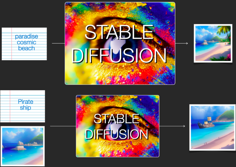
Stable Diffusion 組成元件

Stable Diffusion 是一個系統包含多個組件和模型，而非單一的模型。可以簡單分成兩大塊：文本理解組件和圖像生成組件。

• 文本理解 (text encoder): transformer network 的 encoder 部分
  • 類似 BERT? Not exactly。因爲要同時處理 text and image, 需要 multi-modal vision and language model，比較像是 CLIP (Contrastive Language-Image Pre-Training). Transformer 家族的 BERT, ViT, CLIP, 和 BLIP 的差異可以參考 appenix.
• 圖像生成 (image generator): diffusion network based on U-Net?

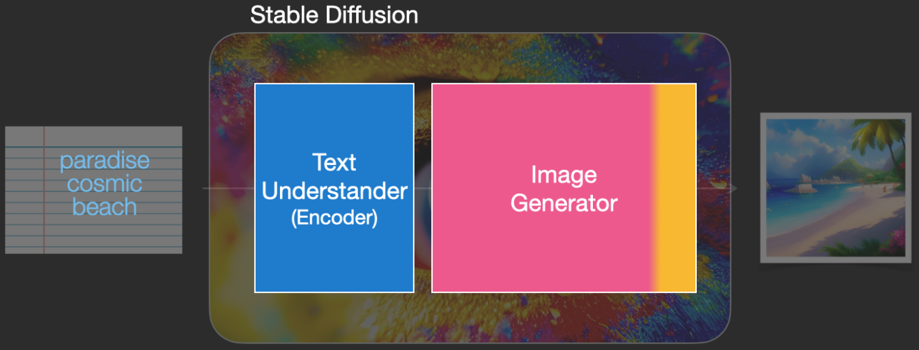
文本理解器 (Text Understander)

將文本信息翻譯成數字表示 (numeric representation)，以捕捉文本中的語義信息。

雖然目前還是從宏觀角度分析模型，之後才有更多的模型細節。但我們可以大致推測這個文本編碼器 (text encoder) 是一個特殊的Transformer model. 具體來說是 CLIP - Contrastive Language-Image Pre-Training 模型的文本編碼器。

我們先考慮文本輸入：模型的輸入為一個文本字元串，輸出為一個數字列表，用來表徵文本中的每個單詞/token，即將每個 token 轉換為一個向量。 然後這些信息會被提交到圖象生成器

圖像生成器 (Image Generator)

圖象生成器主要包括兩個階段：

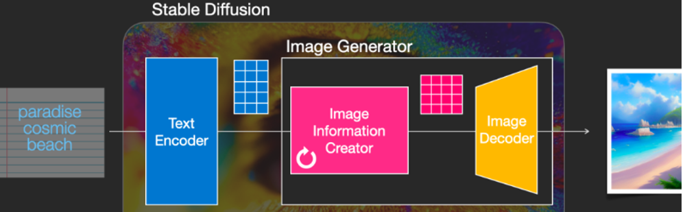
1. Image information creator (latent space)

這個組件是 Stable Diffusion 的獨家秘方。相比之前的模型，它的很多性能改善都是在這個組件實現。 該組件運行多個 denoise steps 來生成圖像信息，其中 steps 也是Stable Diffusion 介面和 library 中的參數，通常預設為 50 或 100。

Image information creator 完全在 image information space（latent space）中運行，這一特性使得它比其他在 pixel space 工作的 Diffusion 模型運行得更快。從技術上來看，該組件由一個 UNet 和一個scheduling 算法組成。

• Scheduling algorithm 是產生高畫質的關鍵！
• UNet 目前面臨 transformer decoder 的挑戰。

Diffusion 描述了在該組件內部運行期間發生的事情，即對 image information (不是 image 本身) 進行一步步地處理，並最終由下一個組件（圖像解碼器）生成高質量的圖象。

2. 圖像解碼器 (Image Decoder)

圖像解碼器根據從 Image Information Creator 中獲取的信息產生出一幅畫。整個過程只運行一次即可生成最終的像素級圖像。這個 decoder 類似 VAE 的 decoder.

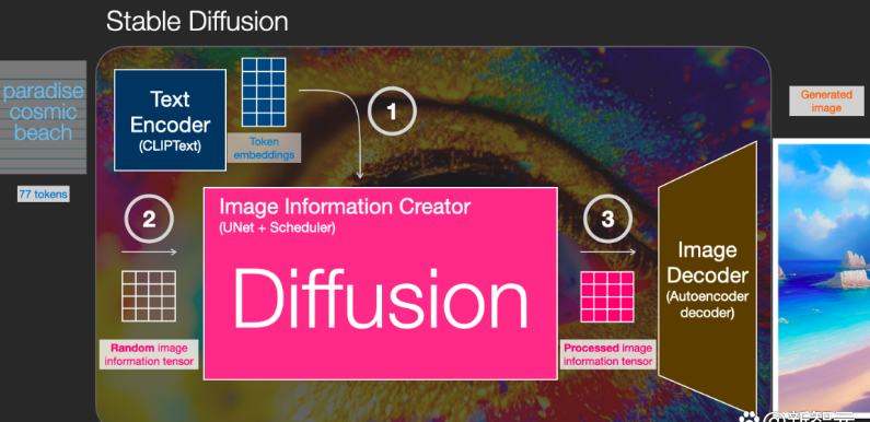
神經網絡模型

可以看到，Stable Diffusion總共包含三個主要的組件，其中每個組件都擁有一個獨立的神經網絡：

• Clip Text 用於文本 (和圖像) 編碼。 輸入：文本 輸出：77 個 token embeddings 向量，其中每個向量包含 768 個維度
• UNet + Scheduler 在 information (latent) space 中逐步處理/擴散信息。 輸入：embeddings 和一個由雜訊初始 tensor. 輸出：一個經過處理的 information tensor.
• 自編碼解碼器（Autoencoder Decoder），使用處理過的 information tensor 繪製最終圖像的解碼器。 輸入：處理過的 information tensor，維度為（4, 64, 64） 輸出：最終圖像，維度為（3，512，512）即（RGB，寬，高）

Diffusion

最關鍵的部分就是 diffusion. Diffusion 是在下圖中粉紅色的 Image Information Creator 組件中發生的過程，過程中包含表徵輸入文本的 (1) token embeddings，和隨機初始的 (2) image tensor（也稱之為 latents），該過程會還需要用到圖象解碼器來繪製最終 (3) 圖象的信息矩陣。

整個運行過程是 step-by-step，每一步都會增加更多的相關信息。 為了更直觀地感受整個過程，可以中途查看隨機 latents 矩陣，並觀察它是如何轉化為視覺雜訊的，其中視覺檢查（visual inspection）是通過圖象解碼器進行的。

整個diffusion過程包含多個steps，其中每個step都是基于輸入的 latents 矩陣進行操作，並生成另一個 latents 矩陣以更貼近「輸入的文本」和從模型圖象集中獲取的「視覺信息」。

將這些 latents 可視化可以看到這些信息是如何在每個 step 中相加的。

整個過程就是從無到有，看起來相當激動人心。

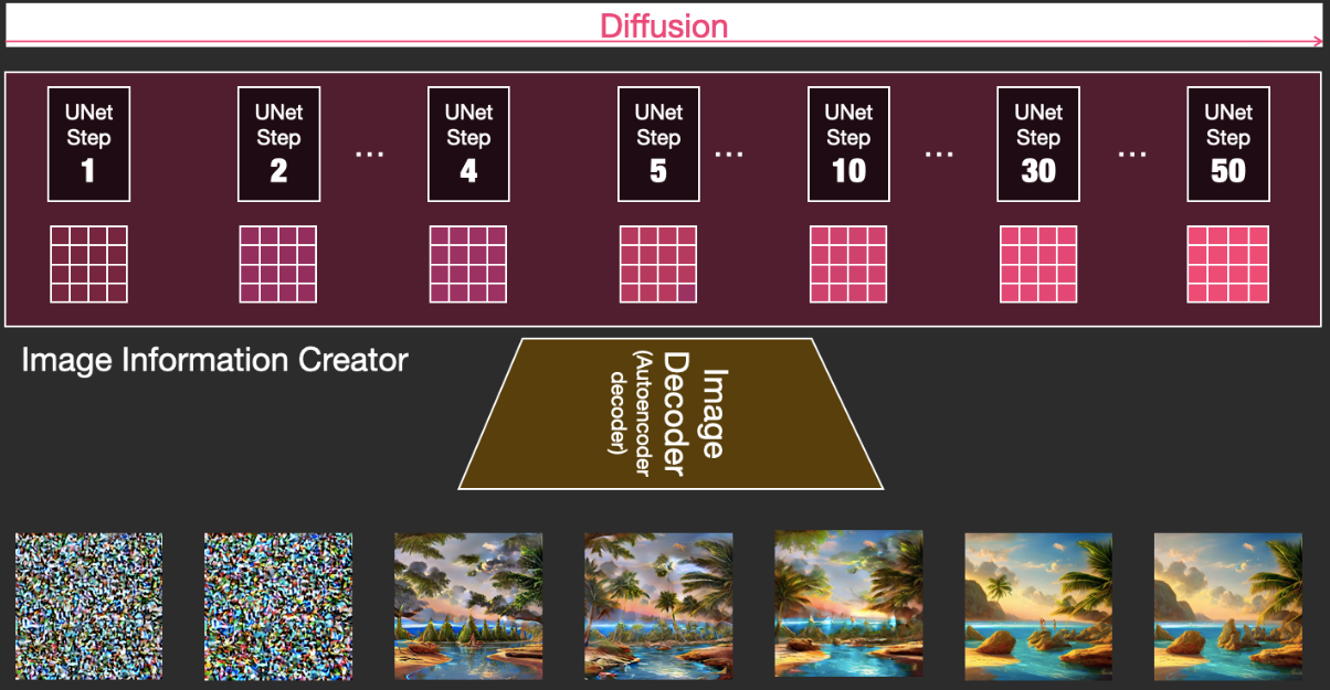
步驟2和4之間的過程轉變看起來特別有趣，就好像圖片的輪廓是從雜訊中出現的。

Diffusion 的工作原理

有兩種觀點：image denoise 或是 noise prediction. 目前是以 noise prediction 爲主, why?

• Predict noise 之後的 loss 計算和 back-propagation 都和原始 image 無關，似乎比較簡單?
• 如果是 image denoise, 結果需要和原始 image 比較 (相減) 的 loss 才能 back-propagation, 比較麻煩?
• 所以這和一般影像的 denoise 或是 predict noise 似乎不同？還是要用影像的 noise 來 train, 而非用 Gaussian noise?

使用擴散模型生成圖象的核心思路還是基于已存在的強大的計算機視覺模型，只要輸入足夠大的數據集，這些模型可以學習任意複雜的操作。

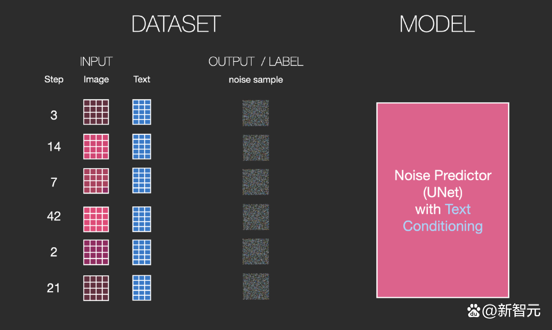
Forward path:

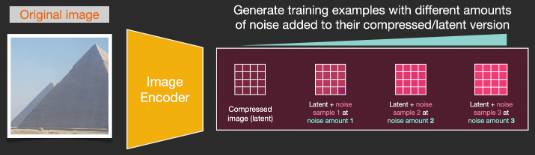
假設我們已經有了一張圖象，生成產生一些雜訊加入到圖象中，然後就可以將該圖象視作一個訓練樣例。

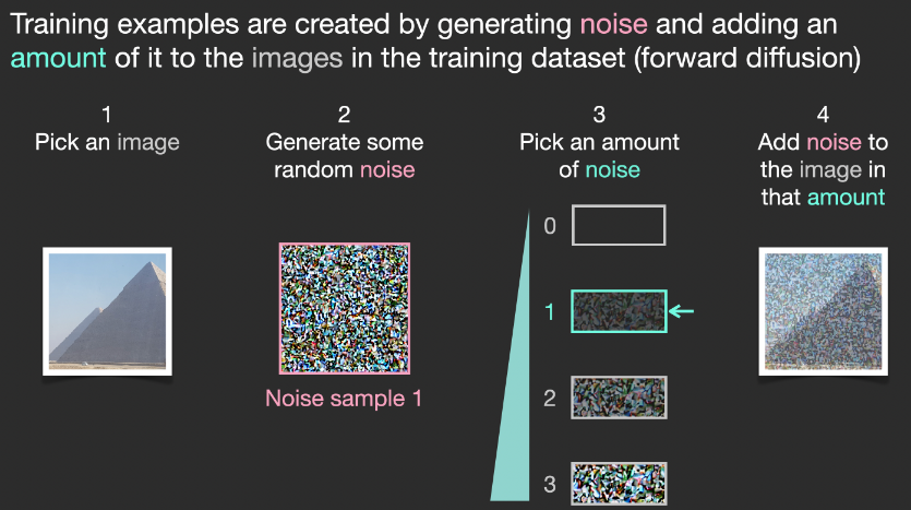
使用相同的操作可以生成大量訓練樣本來訓練圖象生成模型中的核心組件。

這個部分和我的瞭解不同！應該是逐漸加 noise 而非加上不同程度的 noise。還是兩者等價? Yes, 兩者等價: $q(x_t

x_{t-1})$ 是 Gaussian, $q(x_t \vert x_o)$ 也是 Gaussian.

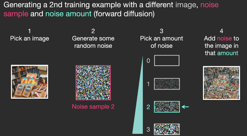
上述例子展示了一些可選的雜訊量值，從原始圖象(級別0，不含雜訊)到雜訊全部添加(級別4) ，從而可以很容易地控制有多少雜訊添加到圖象中。 所以我們可以將這個過程分散在幾十個steps中，對數據集的每張圖象都可以生成數十個訓練樣本。

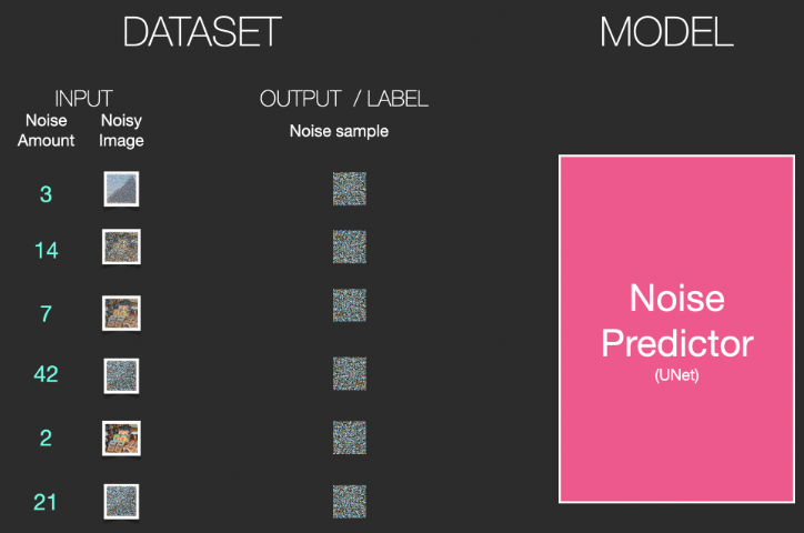
基于上述數據集，我們就可以訓練出一個性能極佳的雜訊預測器，每個訓練 step 和其他模型的訓練相似。當以某一種確定的配置運行時，雜訊預測器就可以生成圖象。

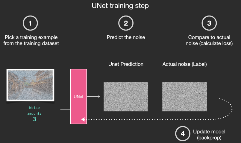
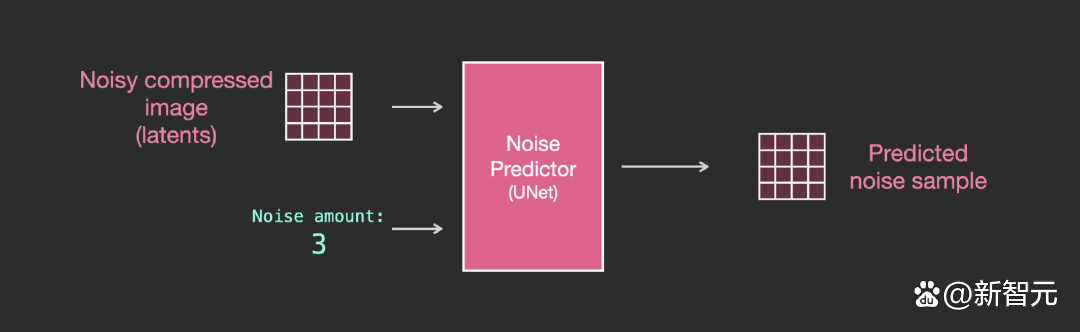
移除雜訊，繪製圖象

經過訓練的雜訊預測器可以對一幅添加雜訊的圖象進行去噪，也可以預測添加的雜訊量。

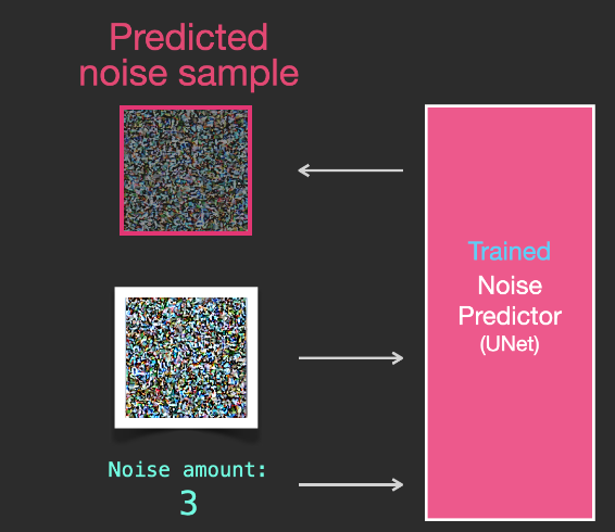
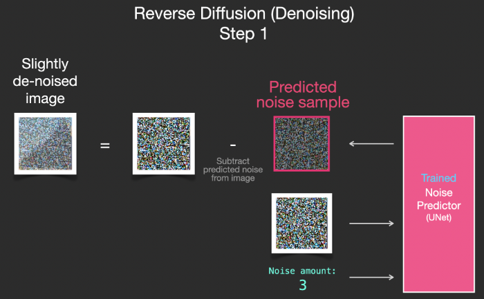
由於採樣的雜訊是可預測的，所以如果從圖象中減去雜訊，最後得到的圖象就會更接近模型訓練得到的圖象。

得到的圖象並非是一張精確的原始圖象，而是分佈（distribution），即世界的像素排列，比如天空通常是藍色的，人有兩隻眼睛，貓有尖耳朵等等，生成的具體圖象風格完全取決於訓練數據集。

以上的步驟成爲 DDPM (Denoising Diffusion Probabilistic Models). 不止Stable Diffusion通過去噪進行圖象生成，DALL-E 2和谷歌的Imagen模型都是如此。

需要注意的是，到目前為止描述的擴散過程還沒有使用任何文本數據生成圖象。因此，如果我們部署這個模型的話，它能夠生成很好看的圖象，但用戶沒有辦法控制生成的內容。 在接下來的部分中，將會對如何將條件文本合併到流程中進行描述，以便控制模型生成的圖象類型。

加速：在壓縮 (Latent) 數據上擴散

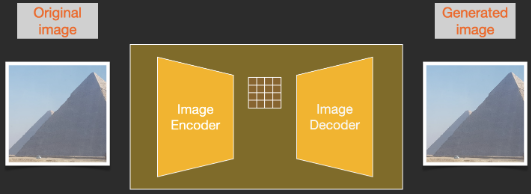
為了加速圖象生成的過程，Stable Diffusion並沒有選擇在像素圖象本身上運行擴散過程，而是選擇在圖象的壓縮版本上運行，論文中也稱之為「Departure to Latent Space」。 整個壓縮過程，包括後續的解壓、繪製圖象都是通過自編碼器 (auto-encoder) 完成的，將圖象壓縮到潛空間中，然後僅使用解碼器使用壓縮後的信息來重構。

前向擴散（forward diffusion）過程是在壓縮latents完成的，雜訊的切片（slices）是應用於latents上的雜訊，而非像素圖象，所以雜訊預測器實際上是被訓練用來預測壓縮表示（潛空間）中的雜訊。

前向過程，即使用使用自編碼器中的編碼器來訓練雜訊預測器。一旦訓練完成後，就可以通過運行反向過程（自編碼器中的解碼器）來生成圖象。

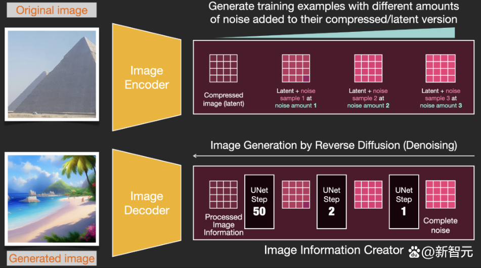
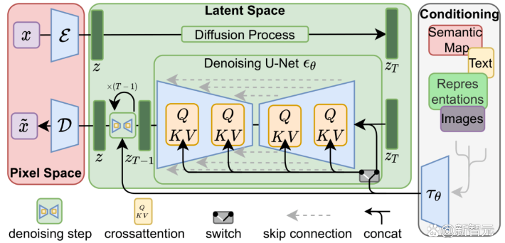
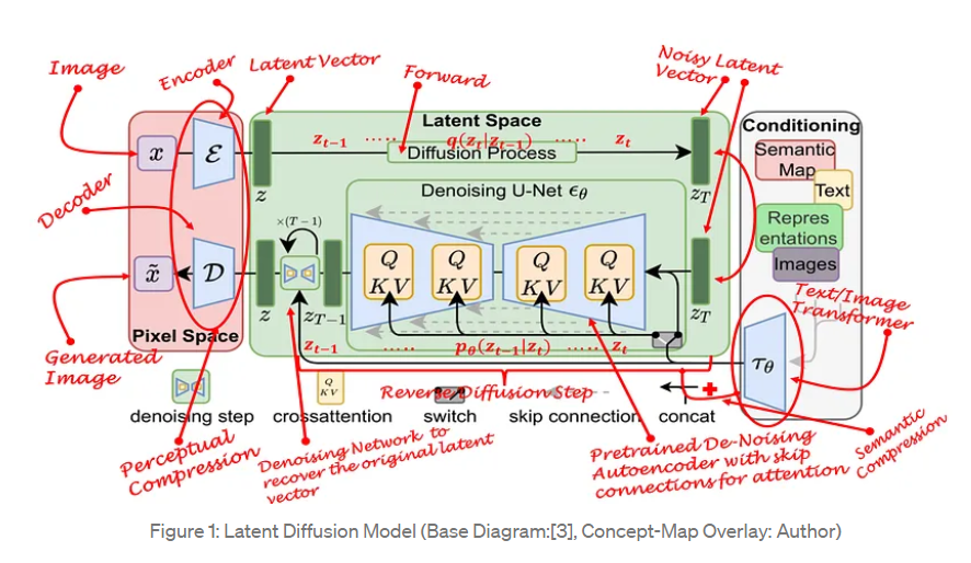
前向和後向過程如下所示，圖中還包括了一個conditioning組件，用來描述模型應該生成圖象的文本提示。

文本編碼器：Transformer 語言模型

模型中的語言理解組件使用的是 Transformer 模型，可以將輸入的 text prompt 轉換為 token embeddings 。發佈的 Stable Diffusion 模型使用 ClipText (基于 GPT 的模型) ，這篇文章中為了方便講解選擇使用 BERT模型。

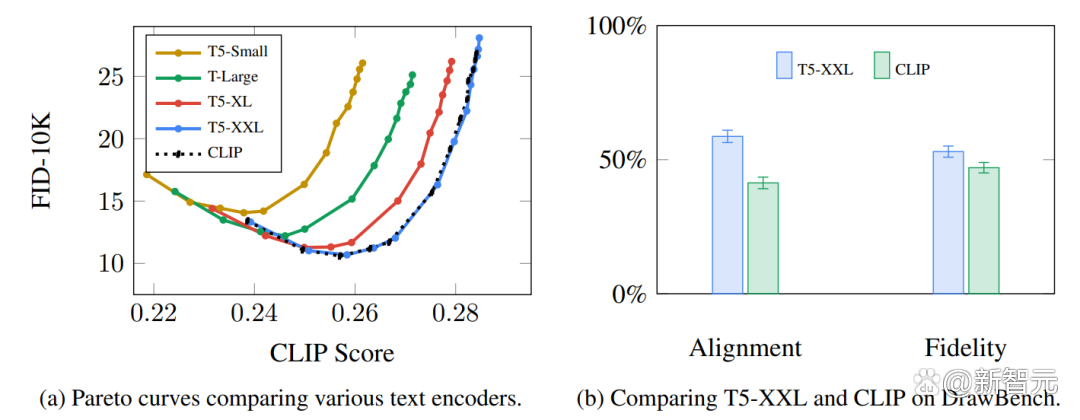
Imagen論文中的實驗表明，相比選擇更大的圖象生成組件，更大的語言模型可以帶來更多的圖象質量提升。

早期的Stable Diffusion模型使用的是OpenAI發佈的經過預訓練的 ClipText 模型 (63M 參數)，而在Stable Diffusion V2中已經轉向了最新發佈的、更大的CLIP模型變體 OpenClip (354M 參數)。

CLIP是怎麼訓練的？

CLIP需要的數據為圖象及其標題，數據集中大約包含400M 張圖象及描述。

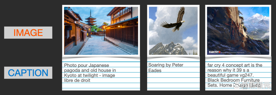
事實上，CLIP 通過從網上抓取的圖片以及相應的「alt」標籤文本來收集 dataset。

CLIP 是圖象編碼器和文本編碼器的組合，其訓練過程可以簡化為用一張圖象和對應文字來說明。我們用兩個編碼器對數據分別進行編碼。

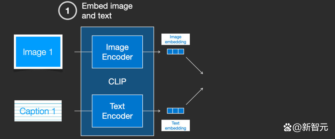
然後使用 cosine similarity 比較結果 embeddings。剛開始訓練時，即使文本描述與圖象是相匹配的，它們之間的相似性肯定也是很低的。

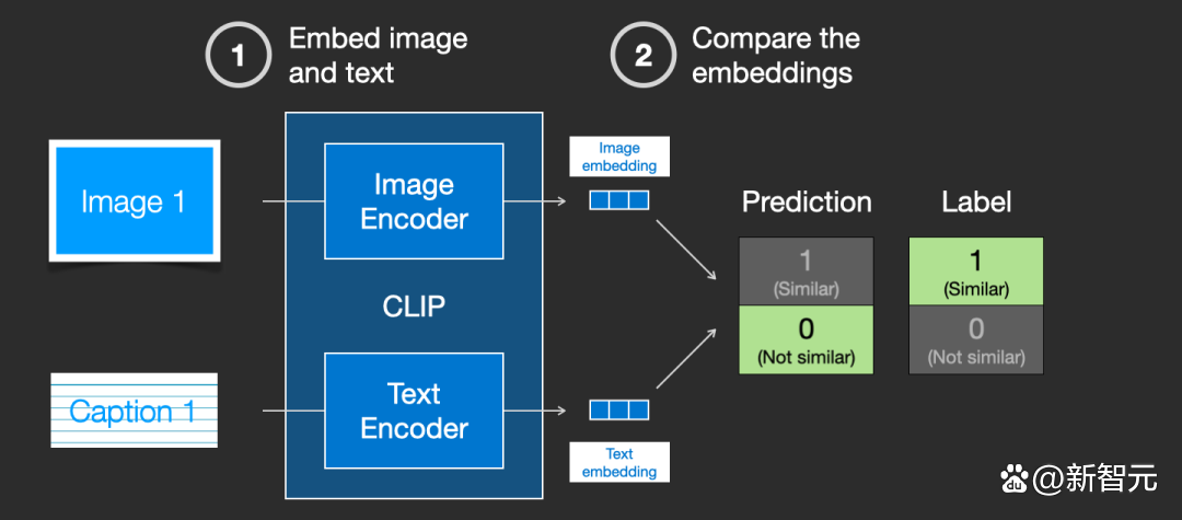
隨著模型的不斷更新，在後續階段，編碼器對圖象和文本編碼得到的嵌入會逐漸相似。

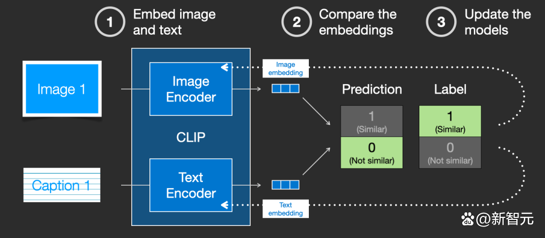
通過在整個數據集中重複該過程，並使用大 batch size，最終能夠生成 joint 編碼器可以產生 embeddings 其中狗的圖象和句子「一條狗的圖片」之間是相似的。就像在 word2vec 中一樣，訓練過程也需要包括不匹配的圖片和說明的負樣本，模型需要給它們分配較低的相似度分數。

文本信息饋入圖象生成過程

為了將文本條件融入成為圖象生成過程的一部分，必須調整雜訊預測器的輸入為文本。

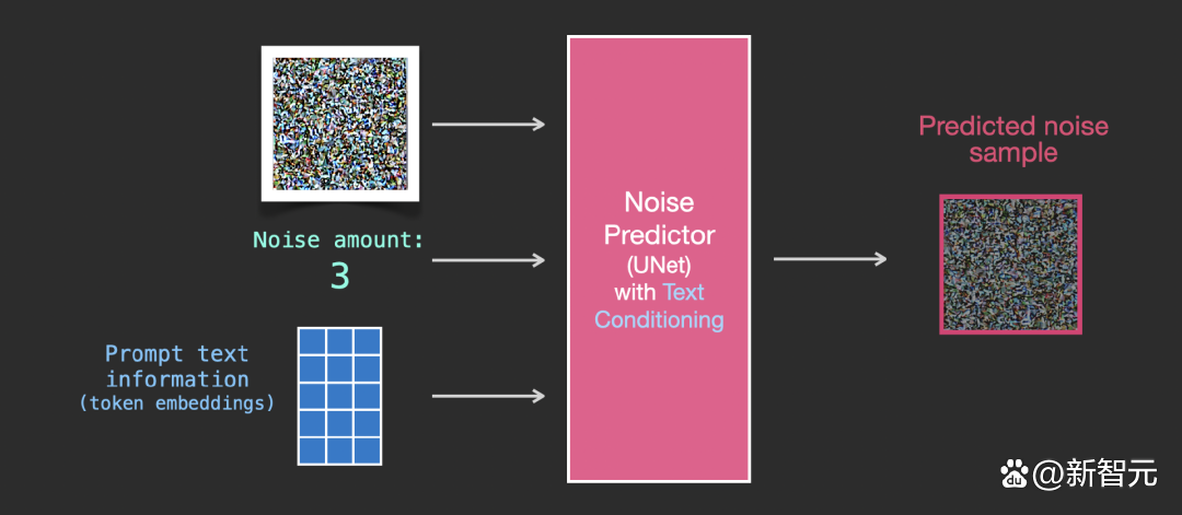
所有的操作都是在潛空間上，包括編碼後的文本、輸入圖象和預測雜訊。

為了更好地瞭解文本token在 Unet 中的使用方式，還需要先瞭解一下 Unet 模型。

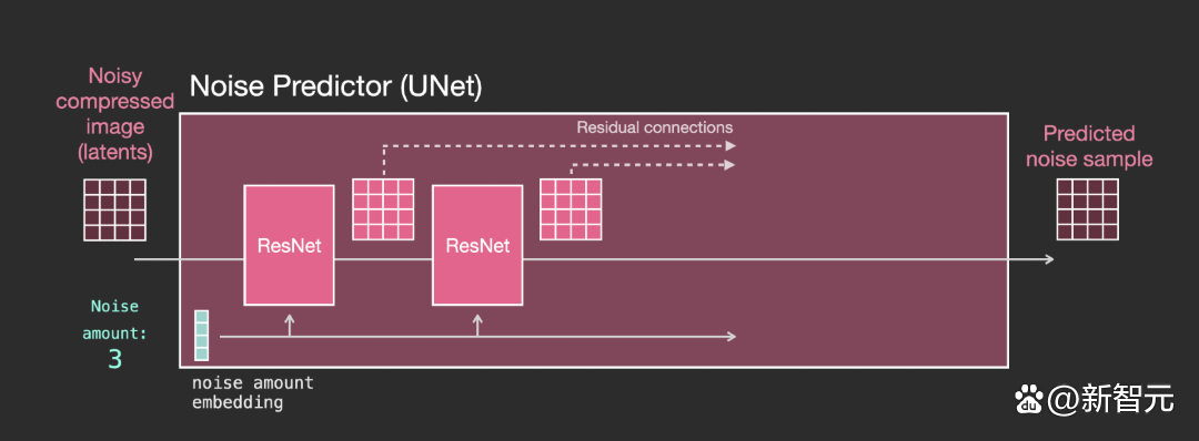
Unet 雜訊預測器中的層（無文本）

一個不使用文本的diffusion Unet，其輸入輸出如下所示：

在模型內部，可以看到：

1. Unet 模型中的層主要用於轉換 latents；
2. 每層都是在之前層的輸出上進行操作；
3. 某些輸出（通過殘差連接）將其饋送到網絡後面的處理中
4. 將時間步轉換為時間步長 embedding vector，可以在層中使用。

Unet 雜訊預測器中的層（帶文本）

現在就需要將之前的系統改裝成帶文本版本的。

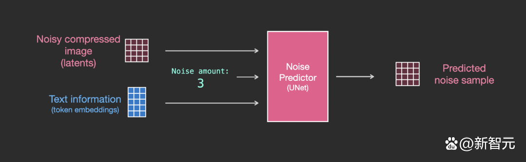
主要的修改部分就是增加對文本輸入（術語：text conditioning）的支持，即在 ResNet 塊之間添加一個注意力層。

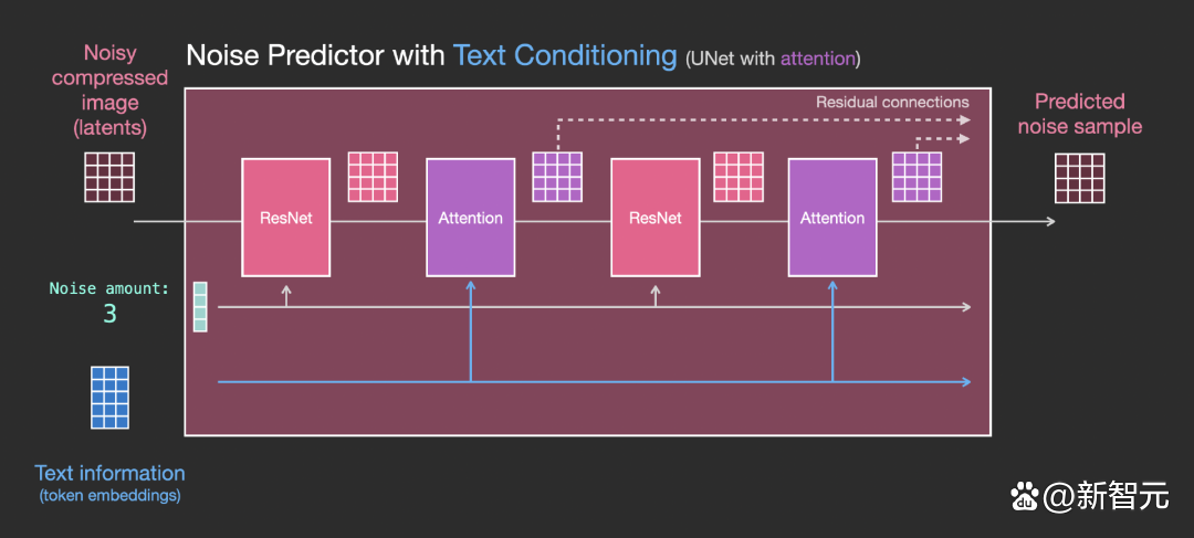
需要注意的是，ResNet塊沒有直接看到文本內容，而是通過 attention layers 將文本在 latents 中的表徵合併起來，然後下一個 ResNet 就可以在這一過程中利用上文本信息。

Appendix

Transformer Family Encoder 比較：ViT, CLIP, BLIP, BERT

Ref: [@jizhiTransformerFamily2022]

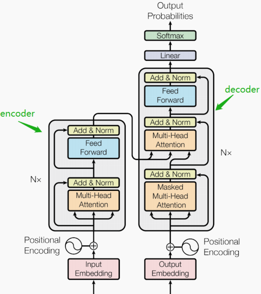
完整的 transformer 包含 encoder (discriminative) 和 decoder (generative).

以下我們主要聚焦於 encoder 部分。因爲 stable diffusion 的 decoder (generative) 部分是由 U-Net 完成的。雖然目前也有 transformer-based 的 decoder.

	Input	Output
Transformer (encoder+decoder)	Text	Text
BERT (encoder)	Text	Token Embeddings
ViT (encoder)	Image	Token Embeddings
CLIP (encoder)	Text & Image	Similarity Score
BLIP (encoder+decoder)	Text & Image	Token Embeddings?

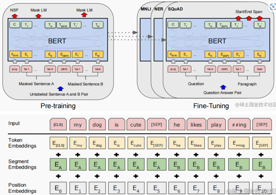
BERT: Bidirectional Encoder Representations from Transformer

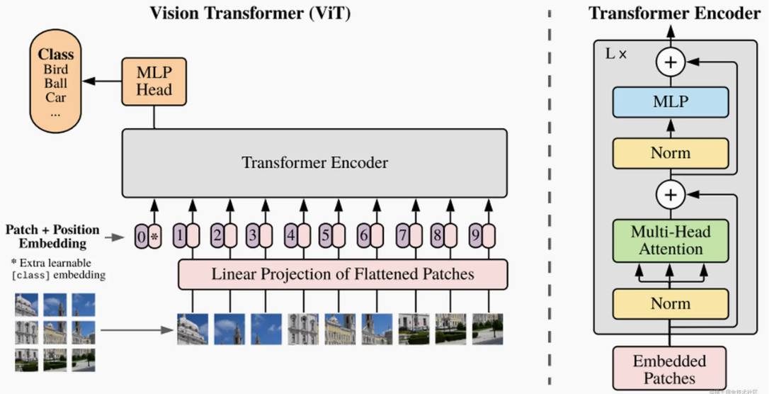
ViT: Vision Transformer Encoder

CLIP: Contrastive Language-Image Pre-Training Encoder

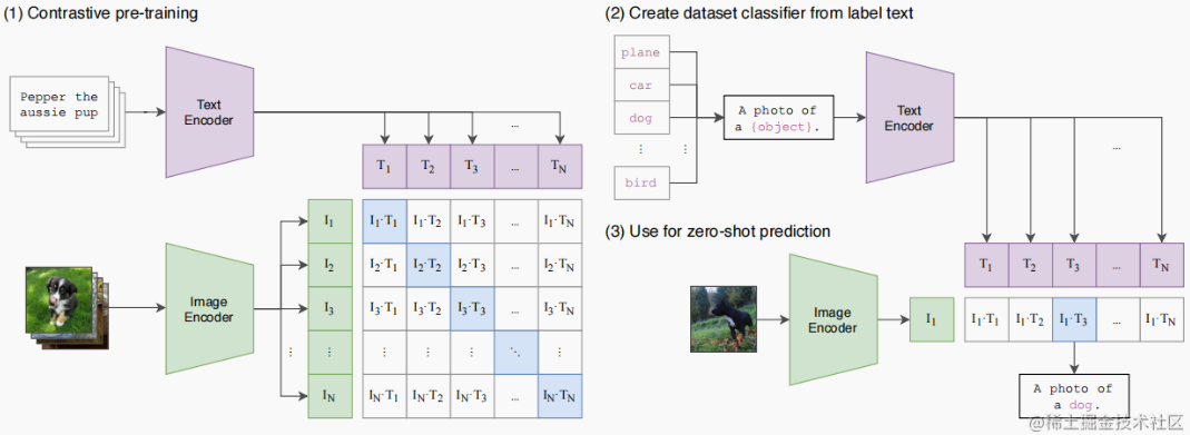
CLIP是一個 multi-modal vison and language model。它可用於 (image-text) 圖像和文本的相似性以及 zero-shot 圖像分類 (見下圖)。CLIP 使用 ViT-like transformer 獲取視覺特徵，並使用因果語言模型 (causal language model) 獲取文本特徵。然後將文本和視覺特徵投影到具有相同維度的 latent space。最後投影圖像和文本特徵之間的内積產生相似性的分數 (score of similarity)。

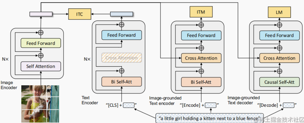
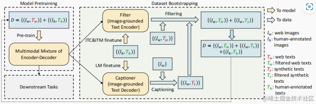
BLIP: Bootstrapping Language-Image Pre-training Encoder/Decoder

Citation