Source
https://allenlu2007.wordpress.com/category/math/
Tensor calculus: (one-form and vector) https://www.youtube.com/watch?v=p75-f0gN5c0&list=PLlXfTHzgMRULkodlIEqfgTS-H1AY_bNtq&index=4&ab_channel=MathTheBeautiful
https://www.seas.upenn.edu/~amyers/DualBasis.pdf : 很好例子
Takeaway
Tensor, (differential) geometry -> manifold -> derivative (differential), connection, xxx -> manifold optimization (conjugate coordinate or conjugate optimization ~ momentum optimization)
- 歐式幾何 (看山是山,純幾何) -> 笛卡爾解析幾何 (看山不是山,坐標系 (代數) 幾何) -> 微分幾何/張量分析 (看山是山,坐標系無關幾何與物理)
-
目標是開創座標系不變 (invariant) 的數學和物理! 兩個步驟:
- Dual/Reciprocal/Biorthogonal basis 就是為了拯救座標系!讓向量和張量的加、減、scaling、內外積在不同坐標系運算仍然可以進行,以達到坐標系不變的結果!
- 不同坐標系的 connection, 也就是微分的關係
- 坐標系不變,但是各個分量卻會是逆變 (contravariant) 或是協變 (covariant). 。判斷的方法很簡單,只要把 basis 變大,如果分量變小就是逆變。如果分量變大就是協變。
- 一般 Vector 的分量是逆變。但是 gradient (梯度) 則是協變。
- Bivector, one-form 都是斜邊。
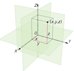
卡氏座標系:不變,協變,逆變
笛卡爾對數學的一大成就是引入 (笛卡爾) 卡氏座標系。把幾何問題轉換並結合成代數問題。
所謂卡氏座標系通常用 $\hat{x},\hat{y},\hat{z}$ 或是 $\mathbf{e}_1, \mathbf{e}_2, \mathbf{e}_3$ (以 3D 為例) 代表基底向量 (basis vectors)。
卡氏座標系的基底向量滿足:(1) 正交座標系;(2) 基底向量是 globally fixed, 不隨空間位置改變。 \(\mathbf{e}_i \cdot \mathbf{e}_j = \delta_{ij} = \begin{cases} 1, & i = j \\ 0, & i \neq j \end{cases}\)
有了基底向量,就可以定義 (vector space) 空間中任意的點 (或是向量) : $\vec{V} = x \mathbf{e}_1 + y \mathbf{e}_2 + y \mathbf{e}_3 = (x, y, z)$. 以及對應的加、減、距離、scaling, inner product, 等等。
- 因為 $x = \vec{V}\cdot \mathbf{e}_1; y = \vec{V}\cdot \mathbf{e}_2; z = \vec{V}\cdot \mathbf{e}_3$ ,所以 $\vec{V} = (\vec{V}\cdot \mathbf{e}_1) \mathbf{e}_1 + (\vec{V}\cdot \mathbf{e}_2 )\mathbf{e}_2 + (\vec{V}\cdot \mathbf{e}_3) \mathbf{e}_3 $
- 簡單說就是把原始向量拆分成各個基底向量的分量。在卡氏座標系的分量就是投影量 。
- 但在非卡氏座標系就不是投影量,如何處理?
注意卡氏座標系並非等價正交座標系!
- 例如 3D 球面上的 tangent plane 也可以定義 2D 正交座標系,但不是 globally fixed。所以不是卡氏座標系。
卡氏座標系雖然結合幾何和代數領域。但有一大缺點:幾何 (以及相關的物理) 問題就和座標系綁在一起!
很多幾何和物理問題的座標系並非卡氏座標系,或並非最適合用卡氏座標系描述 (圓,球)
- 幾何:(非卡氏座標系) manifold 上的微分,積分,optimization
- 物理:不同的觀察者對應不同的 (非卡氏) 座標系
除了描述或觀察的方便,我們更大的目標是:幾何歸幾何;物理歸物理;代數歸代數!
也就是說,很多幾何問題或是物理問題應該和選擇的卡氏或非卡氏座標系無關,例如
- 幾何:球面任意兩點最短的軌跡應該和用什麼座標系不變 (invariant)
- 物理:牛頓定律、狹義相對論、廣義相對論在不同的觀察者 (座標系) 物理定律不變 (invariant)
我們的目標是開創一門座標系無關的數學!如何進行?
Step1: 引入另一組基底向量
Step2: 空間不同位置的座標系之間的 connection! 也就是微分關係!
Step3: 利用新的數學,重新改寫微分幾何和張量分析。還有微積分定理!!!
Step1 : 非卡氏座標系 I (假設 flat space)
Dual/Reciprocal/Biorthogonal/Colinear/Curvilinear/Conjugate Basis
雖然我們的目標是座標系無關,但也有一些幾何或物理量是和座標系相關
- 幾何:空間中一個向量的長度和方向應該是座標系不變,但是其分量和座標軸刻度逆變 (contra-variant)。也就是基底越大,對應的分量越小,才能保證長度不變。
- 物理:伽利略座標系不同觀察者看到的速度顯然不一樣。狹義座標系不同觀察者看到的長度和時間不一樣。
我之前一直不明白為什麼要引入 covariant/contra-variant components, 或是 vector/co-vector, 或是 1/2/3-vector/1/2/3-form, 或是 conjugate coordinate!!! 只是徒添亂。
現在明白 Dual/Reciprocal/Biorthogonal basis 是為了拯救座標系!讓向量和張量的加、減、scaling、內外積在不同坐標系運算仍然可以進行,以達到坐標系無關的結果!
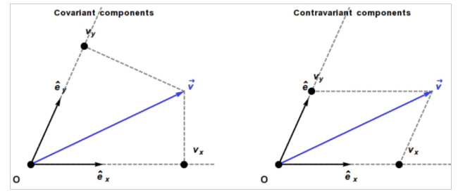
Covariant and Contravariant: 協變和逆變
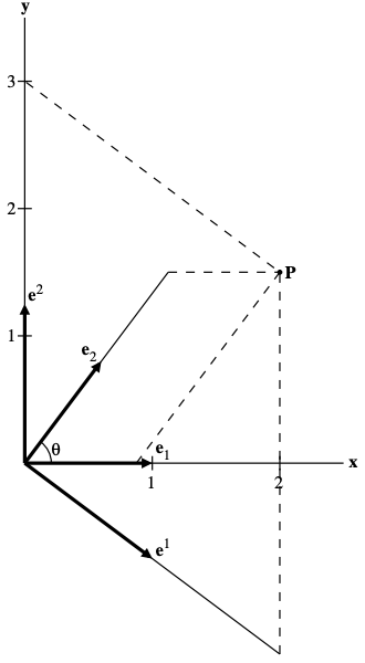
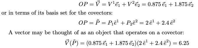
對於非正交坐標系如下圖。如何能得到每個基底向量 (也稱爲 tangent basis) ${\mathbf{e}_1, \mathbf{e}_2}$的分量?
顯然 $\vec{V} \neq (\vec{V}\cdot \mathbf{e}1) \mathbf{e}_1 + (\vec{V}\cdot \mathbf{e}_2 )\mathbf{e}_2$ 因爲 $\mathbf{e}_i \cdot \mathbf{e}_j \neq \delta{ij}$
放在一起:
但是我們可以引入另一組基底向量 ${\mathbf{e}^1, \mathbf{e}^2}$ (也稱爲 cotangent basis), 滿足 \(\mathbf{e}^i \cdot \mathbf{e}_j = \delta^i_j = \begin{cases} 1, & i = j \\ 0, & i \neq j \end{cases}\) 假設 $\vec{V} = X^1 \mathbf{e}_1 + X^2 \mathbf{e}_2 \Rightarrow X^1 = \vec{V}\cdot \mathbf{e}^1 \text{ and } X^2 = \vec{V}\cdot \mathbf{e}^2 $
-
$\vec{V} = X^1 \mathbf{e}1 + X^2 \mathbf{e}_2 = (\vec{V}\cdot \mathbf{e}^1) \mathbf{e}_1 + (\vec{V}\cdot \mathbf{e}^2 )\mathbf{e}_2$ 因爲 $\mathbf{e}^i \cdot \mathbf{e}_j = \delta^i{j}$
- 注意在非正交坐標系 $\mathbf{e}_1 \nparallel \mathbf{e}^1$ 以及 $\mathbf{e}_2 \nparallel \mathbf{e}^2$, 也不要求 $e_i, e^i$ 是 unit vector. 但在正交坐標系 $\mathbf{e}_1 = \mathbf{e}^1$ 以及 $\mathbf{e}_2 = \mathbf{e}^2$
- 如果 $\mathbf{e}_1$ (or $\mathbf{e}_2$) 增加,$\mathbf{e}^1$ (or $\mathbf{e}^2$)減少,因爲 $X^1 = \vec{V} \cdot \mathbf{e}^1$ (or $X^2$) 減少,所以 $X^1, X^2$ 稱爲逆變分量 (contravariant component)
同樣 $\vec{V} = X_1 \mathbf{e}^1 + X_2 \mathbf{e}^2 \Rightarrow X_1 = \vec{V}\cdot \mathbf{e}_1 \text{ and } X_2 = \vec{V}\cdot \mathbf{e}_2 $
- $\vec{V} = (\vec{V}\cdot \mathbf{e}_1) \mathbf{e}^1 + (\vec{V}\cdot \mathbf{e}_2 )\mathbf{e}^2 = X_1 \mathbf{e}^1 + X_2 \mathbf{e}^2$ ; $X_1, X_2$ 稱爲協變分量。
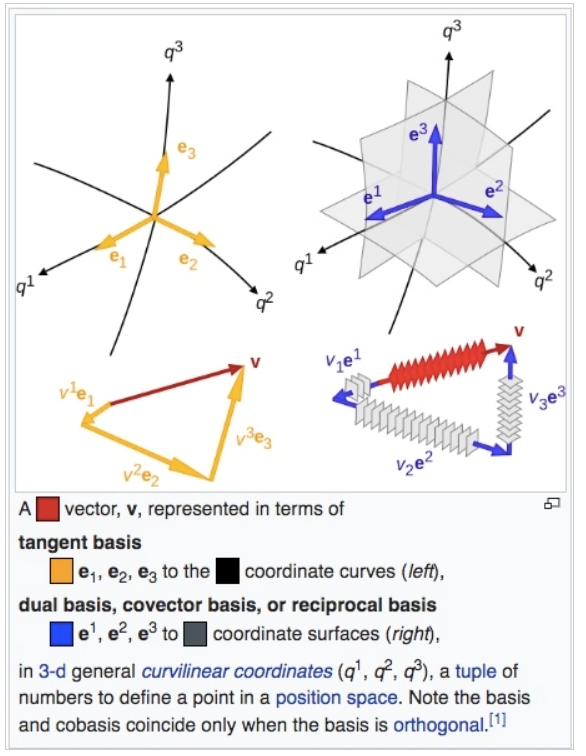
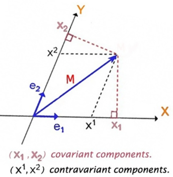
Tensor Analysis/Differential Geometry Dual Basis
對於 tensor analysis / differential geometry,dual basis 的定義:
\[\mathbf{e}^i \cdot \mathbf{e}_j = \delta^i_j\]-
$\mathbf{e}_i$ 稱爲 tangent basis; $\mathbf{e}^i$ 稱爲 cotangent basis
- 一個 vector (tensor) 可以有兩種表示方法,可以用 Einstein notation 簡化
-
$\vec{V} = X_1 \mathbf{e}^1 + X_2 \mathbf{e}^2 = X^1 \mathbf{e}_1 + X^2 \mathbf{e}_2 = X^i \mathbf{e}_i = X_i \mathbf{e}^i$
-
$X^i$ 稱爲 contravariant component; $X_i$ 稱爲 covariant component
-
- 不同的 basis (tangent or cotangent basis),但是描述同一個 vector $\vec{V}$ 或是 tensor.
Geometric Algebra / Clifford Algebra
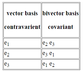
完整的 GA “basis” of geometric algebra 包含 vector $\mathbf{e}_i$, bivector $\mathbf{e}_i \mathbf{e}_j$, tri-vector $\mathbf{e}_i \mathbf{e}_j \mathbf{e}_k$, etc.
以常用 3D “GA basis” $G(3,0)$ 爲例: {1, $\mathbf{e}_1$, $\mathbf{e}_2$, $\mathbf{e}_3$, $\mathbf{e}_1 \mathbf{e}_2$, $\mathbf{e}_2 \mathbf{e}_3$, $\mathbf{e}_3 \mathbf{e}_1$, $\mathbf{e}_1 \mathbf{e}_2 \mathbf{e}_3$ }.
Dual (Vector) Basis
From: [@wikiGeometricAlgebra2023]
Let $ {\mathbf{e}{1},\ldots ,\mathbf{e}{n}}$ be a basis of $V$, i.e. a set of $n$ linearly independent vectors that span the $n$-dimensional vector space. The dual basis is the set of elements of the dual vector space $V^{*}$ that forms a biorthogonal system with this basis, thus being the elements denoted ${\mathbf{e}^{1},\ldots ,\mathbf{e}^{n}}$ satisfying \(\mathbf{e}^i \mathbf{e}_j = \delta^i_j\) 這和 tensor analysis 的 dual basis 定義相同。但如何找到 dual vector basis 和 GA basis 的關係?
Q: 此處應該是假設 $ {\mathbf{e}{1},\ldots ,\mathbf{e}{n}}$ 是 orthogonal basis? $\mathbf{e}_i \mathbf{e}_j = \mathbf{e}_i \wedge \mathbf{e}_j$ for $i \ne j$
-
$\mathbf{e}_1 \wedge \mathbf{e}_2 \wedge \mathbf{e}_3 = I$ (or $i$),$I^2=i^2=-1$ 稱爲 pseudo-scalar.
-
$\mathbf{e}^i = (-1)^{i-1} (\mathbf{e}_1 \wedge \ldots \wedge \hat {\mathbf{e}}_i \wedge \ldots \wedge \mathbf{e}_n) I^{-1}$ where $\hat{\mathbf{e}}_i$ 代表 $i$-th basis vector 被省略。
- 可以檢查: $\mathbf{e}^i \mathbf{e}_i = +1$,以及 $\mathbf{e}^i \mathbf{e}_j = 0$ for $i \ne j$.
-
以 3D GA 爲例:
-
$\mathbf{e}^1 = (\mathbf{e}_2 \wedge \mathbf{e}_3) (\mathbf{e}_1 \wedge \mathbf{e}_2 \wedge\mathbf{e}_3)^{-1} = -i \mathbf{e}_2 \wedge \mathbf{e}_3 = -i \mathbf{e}_2 \mathbf{e}_3 $
- $\mathbf{e}^2 = -(\mathbf{e}_1 \wedge \mathbf{e}_3) (\mathbf{e}_1 \wedge \mathbf{e}_2 \wedge\mathbf{e}_3)^{-1} = i \mathbf{e}_1 \wedge \mathbf{e}_3 = i \mathbf{e}_1 \mathbf{e}_3 = -i \mathbf{e}_3 \mathbf{e}_1$
- $\mathbf{e}^3 = (\mathbf{e}_1 \wedge \mathbf{e}_2) (\mathbf{e}_1 \wedge \mathbf{e}_2 \wedge\mathbf{e}_3)^{-1} = -i \mathbf{e}_1 \wedge \mathbf{e}_2 = i \mathbf{e}_2 \mathbf{e}_1 = = -i \mathbf{e}_1 \mathbf{e}_2$
- 如果忽略 pseudo-scalar $i$ or $-i$, 可以得到以下的 (covariant) bivector basis. 不過如果要把 vector 分解成 covariant bivector basis, 還是要乘 $-i$ 才能把 bivector 轉換成 vector!
-
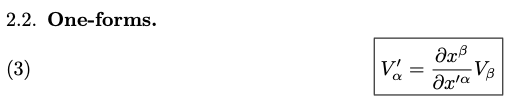
One-Form
(One-Form = Bivector = Covariant Vector)
https://www.quora.com/What-is-the-physical-geometric-difference-between-a-vector-and-its-associated-one-form#:~:text=What%20is%20the%20difference%20between%20%22one%20form%22%20and%20a%20vector,are%20at%20the%20beginning%20level.)
One-forms are basically bivectors (that is, covariant vectors).
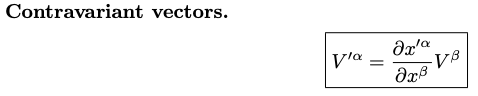
An ordinary vector which takes a point to some other point must transform contravariantly (naively: if you increase your unit of length, the numerical values of the components of a contravariant vector or tensor must decrease correspondingly.) This would be a position vector, denoted (in the indexed notation) using upper indices, like $x^i$
The same applies to velocities; if you have an independent time coordinate 𝜏 (ordinary time in nonrelativistic physics, or proper time in relativistic physics), the velocity will be 𝑣𝑖=𝑑𝑥𝑖/𝑑𝜏. again contravariant.
In contrast, a gradient field (i.e., a force) would end up with the contravariant coordinate in the denominator: that is, ∂𝑖=∂/∂𝑥^𝑖 transforms as a covariant quantity.
Similarly, the canonical definition for four-momentum is given by 𝜋𝑖=∂𝐿/∂𝑣^𝑖. So the “natural” way to present momentum would be as covariant vectors, i.e., as one-forms.
Q3: vector vs. form; or vector vs. chain 微積分
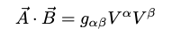
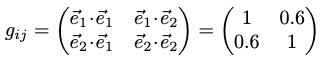
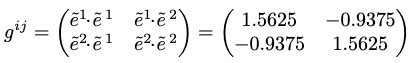
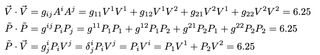
度規 (Metric) 矩陣和 Distance
度規聽起來是個高大上的詞。其實就是 basis vector 的內積矩陣,如下公式。[@myersGENERALRELATIVITY2002]
如果是卡式 (正交且平直) 座標系,三個公式完全一樣,metric 就是 1 or 0。但是在非卡式座標系 (非正交或是非平直) metric 變有趣,非 1 or 0. \(\mathbf{e}^i \mathbf{e}_j = \delta^i_j\)
\[\mathbf{e}_i \mathbf{e}_j = g_{ij}\] \[\mathbf{e}^i \mathbf{e}^j = g^{ij}\]距離或內積
Vector to vector, or covector to convector
Convector to Vector
幾個例子:
非正交但平直座標系度規矩陣。因為度規矩陣是對稱矩陣,所以 eigenvalues 為實數,也就是非旋轉空間。
狹義相對論 (非正交但平直) 時空度規 $(x,y,z,t)$, 非常接近卡氏座標系。
$G=\left(\begin{array}{cc}
1 & 0 & 0 & 0
0 & 1 & 0 & 0
0 & 0 & 1 & 0
0 & 0 & 0 & -1
\end{array}\right)$
曲率張量 (Curvature)
曲率可以判斷是否為平直空間。曲率基本是度規 (metric) 的微分。因為度規是矩陣,所以廣義的曲率是張量。
如果度規矩陣隨位置改變 (放大/縮小或是旋轉) 則度規微分對應的曲率不為 0,代表是彎曲空間。反之如果度規微分為 0, 代表曲率為 0,也就是平直空間。
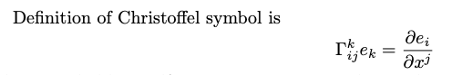
我們會先定義 tangent vector 的微分,稱為 Christoffel symbol. 然後推導度規矩陣的微分。
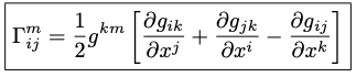

- 如果度規矩陣微分為 0, Christoffel symbol 為 0. Riemann curvature 也為 0. Ricci scalar curvature 為 0.
Step 2: 非卡氏座標系 II: Connection (微分)
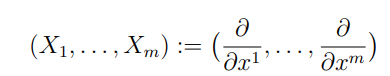
Connection 有很多種,我們先看一種 Christoffel connection。考慮 $T_p M$ (tangent space) over $U$. $\Phi = (X_1, \ldots, X_m)$ 是 basis of the $T_p M$.
There are smooth functions $\Gamma^k_{ij}:U \to \mathbf{R}, 1 \le i,j,k \le m$, such that \(D_{X_i} X_j = \Gamma^k_{ij} X_k\) Connection 的分量 $\Gamma^k_{ij}$ 稱爲 Christoffel symbol of $D$ with respect to $\Phi$.
其他的像是 Affine connection, Levi-Civita connection, Cartan connection.
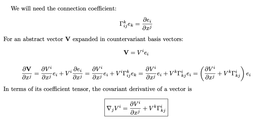
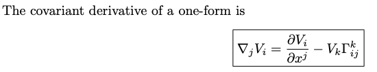
Covariant Derivative
曲率張量 (Curvature)
曲率可以判斷是否為平直空間。曲率直覺是 tangent basis vector 的二次微分。
我們先定義 tangent vector 的一次微分,稱為 Christoffel symbol。Christoffel symbol 是一種 connection.
因為度規是 tangent vector 的微分,可以把 Christoffel symbol 轉換成度規矩陣的微分。
曲率基本是 connection (Christoffel symbol) 的一次微分,等效於 tangent basis vector 的二次微分
- 如果度規矩陣隨位置改變 (放大/縮小或是旋轉) 則度規微分對應的曲率不為 0,代表是彎曲空間。
- 反之如果度規微分為 0, Christoffel symbol 為 0. 代表曲率 (Riemann/Ricci curvature) 為 0,也就是平直空間。
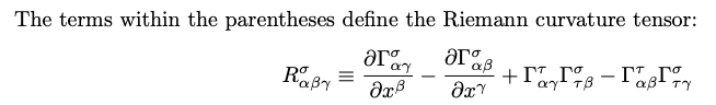
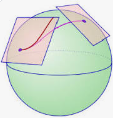
直接二次微分 (Parallel Transport)
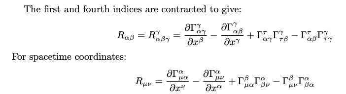
Parallel transport of a vector is defined as transport for which the covariant derivative is zero. The Riemann tensor is determined by parallel transport of a vector around a closed loop. Consider the commutator of covariant differentiation of a one-vector: \(\left[\nabla_\gamma \nabla_\beta-\nabla_\beta \nabla_\gamma\right] V_\alpha\) In a flat space, the order of differentiation makes no difference and the commutator is zero so that any non-zero result can be attributed to the curvature of the space. \(\begin{aligned} & \nabla_\beta V_\alpha=\frac{\partial V_\alpha}{\partial x^\beta}-\Gamma_{\alpha \beta}^\sigma V_\sigma \equiv V_{\alpha \beta} \\ & \nabla_\gamma V_\alpha=\frac{\partial V_\alpha}{\partial x^\gamma}-\Gamma_{\alpha \gamma}^\sigma V_\sigma \equiv V_{\alpha \gamma} \\ & \nabla_\beta \nabla_\gamma V_\alpha=\frac{\partial V_{\alpha \beta}}{\partial x^\gamma}-\Gamma_{\alpha \gamma}^\tau V_{\tau \beta}-\Gamma_{\beta \gamma}^\eta V_{\alpha \eta} \\ & =\frac{\partial^2 V_\alpha}{\partial x^\gamma \partial x^\beta}-\frac{\partial \Gamma_{\alpha \beta}^\sigma}{\partial x^\gamma} V_\sigma-\Gamma_{\alpha \beta}^\sigma \frac{\partial V_\sigma}{\partial x^\gamma}-\Gamma_{\alpha \gamma}^\tau\left(\frac{\partial V_\tau}{\partial x^\beta}-\Gamma_{\tau \beta}^\sigma V_\sigma\right)-\Gamma_{\beta \gamma}^\eta\left(\frac{\partial V_\alpha}{\partial x^\eta}-\Gamma_{\alpha \eta}^\sigma V_\sigma\right) \\ & \nabla_\gamma \nabla_\beta V_\alpha=\frac{\partial V_{\alpha \gamma}}{\partial x^\beta}-\Gamma_{\alpha \beta}^\tau V_{\tau \gamma}-\Gamma_{\gamma \beta}^\eta V_{\alpha \eta} \\ & =\frac{\partial^2 V_\alpha}{\partial x^\beta \partial x^\gamma}-\frac{\partial \Gamma_{\alpha \gamma}^\sigma}{\partial x^\beta} V_\sigma-\Gamma_{\alpha \gamma}^\sigma \frac{\partial V_\sigma}{\partial x^\beta}-\Gamma_{\alpha \beta}^\tau\left(\frac{\partial V_\tau}{\partial x^\gamma}-\Gamma_{\tau \gamma}^\sigma V_\sigma\right)-\Gamma_{\gamma \beta}^\eta\left(\frac{\partial V_\alpha}{\partial x^\eta}-\Gamma_{\alpha \eta}^\sigma V_\sigma\right) \\ & \end{aligned}\) Each equation has 7 terms. In the commutator, the first terms cancel because the order of normal partial derivatives does not matter. The 3rd term of the first equation cancels with the 4th term of the second equation because the symbols used for dummy indices are irrelevant. The 4th term of the first equation cancels with the 3rd term of the second equation for the same reason. The 6th and 7 th terms cancel because Christoffel symbols are symmetric in their lower indices. Only the 2nd and 5th terms survive: \(\left[\nabla_\gamma \nabla_\beta-\nabla_\beta \nabla_\gamma\right] V_\alpha=\left(\frac{\partial \Gamma_{\alpha \gamma}^\sigma}{\partial x^\beta}-\frac{\partial \Gamma_{\alpha \beta}^\sigma}{\partial x^\gamma}+\Gamma_{\alpha \gamma}^\tau \Gamma_{\tau \beta}^\sigma-\Gamma_{\alpha \beta}^\tau \Gamma_{\tau \gamma}^\sigma\right) V_\sigma\) The terms within the parentheses define the Riemann curvature tensor: \(R_{\alpha \beta \gamma}^\sigma \equiv \frac{\partial \Gamma_{\alpha \gamma}^\sigma}{\partial x^\beta}-\frac{\partial \Gamma_{\alpha \beta}^\sigma}{\partial x^\gamma}+\Gamma_{\alpha \gamma}^\tau \Gamma_{\tau \beta}^\sigma-\Gamma_{\alpha \beta}^\tau \Gamma_{\tau \gamma}^\sigma\)