用 Fake coin hypothesis 思考 information theory 如何使用非 constructive method to prove things.
Shannon 的證明有點像鴿籠原理。只證明存在性。
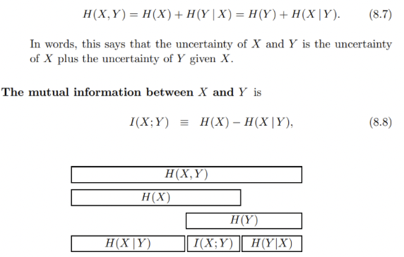
Major Reference and Summary
book.pdf (inference.org.uk) Chap 8-11 from MacKay 是經典 information theory textbook.
(1) High Probability Set vs Typical Set - YouTube
Jointly typical sequences - Microlab Classes (up-microlab.org)
重點
- Noisy but memoryless channel
-
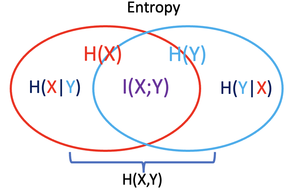
Channel capacity = max mutual information: $\max I(X; Y)$ and $I(X;Y)= H(X) - H(X Y)$. -
$I(X;Y)= H(X)-H(X Y)$ 比起 $H(X)+H(Y)-H(X,Y)$ 更有清晰 insight. 例如 indepedent $X, Y \to H(X Y)=0$ ; 完全 dependent $X,Y \to H(X Y) = 0$.
-
-
Jointly typical set: $2^{nH(X)} 2^{nH(Y X)}$ and $H(X,Y) = H(X) + H(Y X)$ -
所以 jointly typical set (and AEP): $2^{nH(X)} 2^{nH(Y X)} = 2^{nH(X,Y)}$
-
- 低於 channel capacity, 理論上存在 channel code 可以達到 error free communication!
Information Theory Applications
Shannon 的信息論 (Information Theory) 主要包含兩個部分:
| Information | Source | Noisy Channel |
|---|---|---|
| Application | Compression | Communication |
| Source/Channel Capacity |
Source entropy: $H(X)$ | Max source/receiver mutual-info: $\max I(X;Y)$ |
| Shannon Theory | Source Coding Theorem | Channel Coding Theorem |
本文聚焦在 channel code 也就是 communication over noisy channel.
- 從應用面: 一是關於 source encoding/decoding (compression), 另一是關於 channel encoding/decoding (communication over noisy channel)
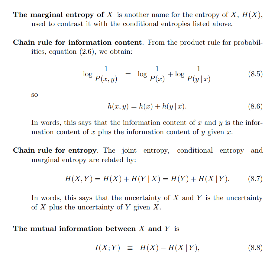
- 從數學面: 一是 self-entropy H(x), 另一是 joint-entropy and mutual information H(x, y), I(X; Y)
第一部分 source encoding for compression 比較容易理解
- 信息 (information) 是不確定性 (uncertainty) 的度量。如果要滿足一些基本特性: Inf = log (1/p(x)), total information = E(Inf) = sum ( p log 1/p)
- 對於 lossy compression 使用 fixed length message , 可以證明 N 夠大,可以 recovery the lossy compress to arbitrary small. 這主要是用於理論推導。實務上雖然有 lossy compression (e.g. jpeg, mp3) 不過大多是 variable length (VBR); 即使有 constant length (CBR) 也是 global 而非 local.
- 對於 lossless compression 使用 variable length message. 理論上有機會達到 H(x), e.g. Hufmann code, LZ code.
- In summary Shannon theory of compression: ? compression rate ~ H(x) ?
第二部分 channel encoding for communication over noisy channel 比較困難
-
對於 noisy channel, 先定義 mutual information:
-
$I(X;Y) = H(X) - H(X Y)$ -
Channel capacity: $C = \max_X I(X;Y)$
- For AWGN channel : $C = B \log_2 (1 + SNR)$ 此處 B: bandwidth, SNR: signal-to-noise ratio
-
-
Shannon channel code theorem : error-free communication over noisy channel if R < C.
- 這其實違反直覺!直覺上要控制 Pe 任意小,transmission rate 也任意小。 Shannon 厲害的地方在於他不同的看法和推理。就像 Galileo/Newton 的運動定律:沒有外力,物體保持慣性而非靜止。
- 證明非常特別!就像鴿籠原理,不是 constructive proof,而是用機率 (大數法則) 只證明存在性。
- 第一部分和 source compression 一樣。找出 $X^n$ 的 typical set ~ $2^{n H(X)}$
-
第二部分比較特別是造出 $(X^n, Y^n)$ jointly typical set ~ $2^{n H(X)} 2^{n H(Y X)} = 2^{n H(X,Y)}$ -
最後找出 non-confusable subset ~ $2^{nH(X)}/2^{nH(X Y)}=2^{nI(X;Y)}$ Non-confusable subset 的 average entropy = $\log_2 2^{n I(X;Y)}/n = I(X;Y)$ 就是 mutual information.
Communication Over Noisy Channel
Communication over noisy channel encode/decode 如下圖。Encode 加入冗余 (redundancy) 對抗 noisy channel 造成的 errors. Decoder 計算 parity/syndrome 或是用其他方法 (e.g. Viterbi) 糾正錯誤。這種 encode/decode 方式稱為 channel coding, 或是 FEC (Forward Error Correction).
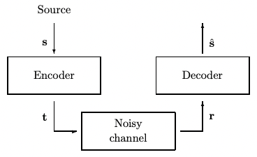
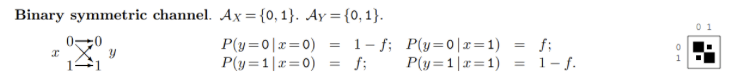
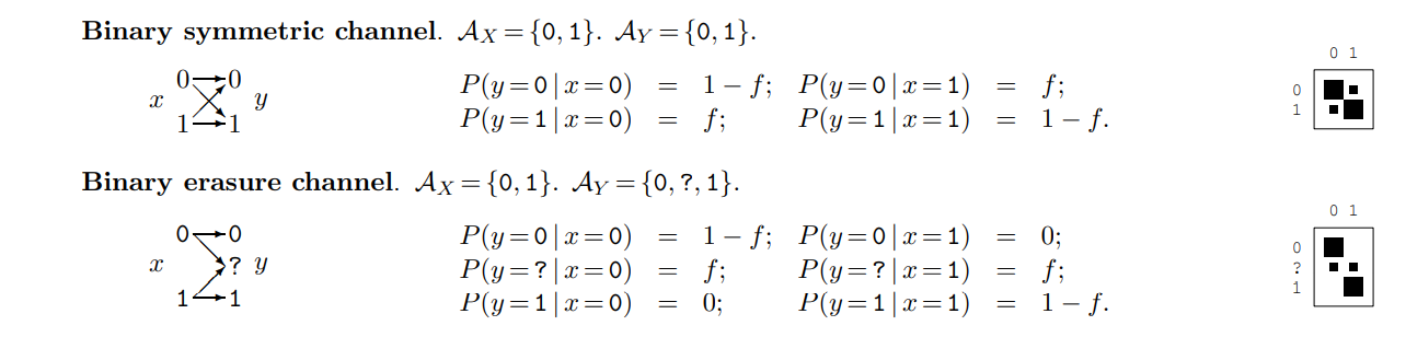
一個最常見的 noisy channel 例子是 BSC (Binary Symmetric Channel), 定義如下。$f$ 代表錯誤的機率。
如何實現 channel coding? 我們先用直觀的方法。再說明 Shannon 的 (天才) 方法。
直觀 Channel Code
Insight From Repetitive Code
最簡單直觀的 channel code 就是 Repetitive code:encoder 就是重複奇數次的 source symbols. decoder 就是 majority vote 決定正確的 symbol. 例如 s = “Alice”; encoder 的 t = “AAAllliiiccceee”。經過 noisy channel 得到 r = “ACAllgiiiaccefe”。Decoder 的 majority vote (所以 encode 要奇數次) 得到 s’ = “AAAllliiiccceee”.
假設 BSC 的錯誤率是 10%, i.e. $f=0.1$. 使用 $k$ (奇數) 次 repetitive code, $R_k$, 對於 error rate 降低的效果如下圖。下圖左是 transmission rate vs. error ratio in linear scale, 下圖右是 transmission rate vs. error ratio in log scale. R1 對應 transmission rate=1, error ratio=0.1. R3 對應的 transmission rate = 0.33, error ratio ~ 0.01.
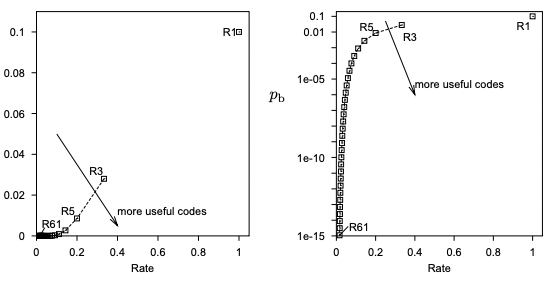
雖然 Repetitive code 非常簡單卻不實用,不過提供 (可能錯誤的) insights!
-
Redundancy (冗余) 可以減少 error ratio.
-
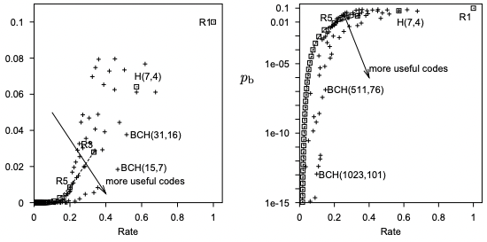
要達到非常小 error ratio (e.g. $10^{-15}$), redundancy 也要愈多 (e.g. R61),transmission rate 也會非常接近 0 (1/61 = 0.016). 更好的 error correction codes 只是讓曲線往 repetitive code 右下方移動。如下圖的 Hamming code, H(7,4), 或是 BCH code.
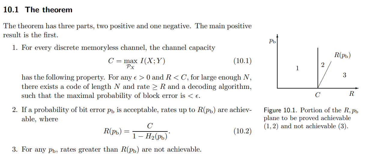
Shannon Channel Code Theory Against Insight
-
要達到任意小的 error rate, 似乎要付出的代價是任意低的 transmission rate. 就是所有的 code 在上圖左都會無限接近 (0,0)。 Shannon 石破天驚推翻這個 insight!
-
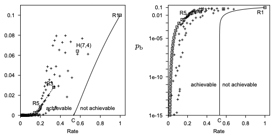
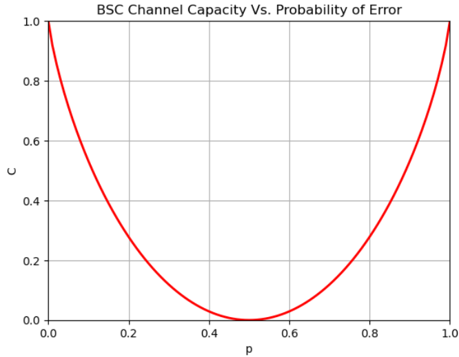
Shannon 定義且計算 channel capacity, C, 就是 achievable 和 not achievable 的 transmission rate 邊界,如下圖。高於 C, 一定無法達成 error free communication. 重點是低於 C, 理論上存在 channel code 可以達到 error free communication!
-
對於 BSC with $f=0.1 \Rightarrow C = H(X)+H(Y)-H(X,Y) = 1+1-1.469=0.531$-bit
-
也就是說,下圖實線右邊是無法達到 error free communication. 但是實線左邊理論上存在 FEC 可以達到 error free communication. 可以看出圖上的 codes (repetitive code, Hamming code, BCH code) 在 low error rate 都離 Shannon capacity 有相當的距離。
-
再強調,令人驚訝的是 C 只有在 error rate 比較大 (>0.01) 時有 linear dependency. 但是在 low error rate (<0.01), C=0.531 基本和 error rate 無關。也就是 error free communication.
接下來我們先說明 Shannon 的結論,這部分很容易。再來試著說明如何達到這個結論,比較抽象。一般稱為 non-constructive proof, 就是證明存在這樣的 code, 但並沒有說明如何造出這個 code.
Joint Entropy, Mutual Information, Capacity
-
注意 : transition probability matrix 和 joint probability distribution 是不同的東西!算 channel capacity 不要搞錯!
-
P(x,y) = p(y x) p(x) 所以會 depends on p(x), 如果 p(x) 是 uniform distribution, 則 p(x,y) ~ p(y x) joint probability ~ transition probability. -
計算 I(X;Y) = H(X) + H(Y) - H(X,Y) , 此處 H(X,Y) 是由 joint probability 決定。
-
也可以用 I(X;Y) = H(X) - H(X Y) = H(Y) - H(Y X), 此處 H(Y X) 則是用 transition probability 決定。後面有幾個例子。
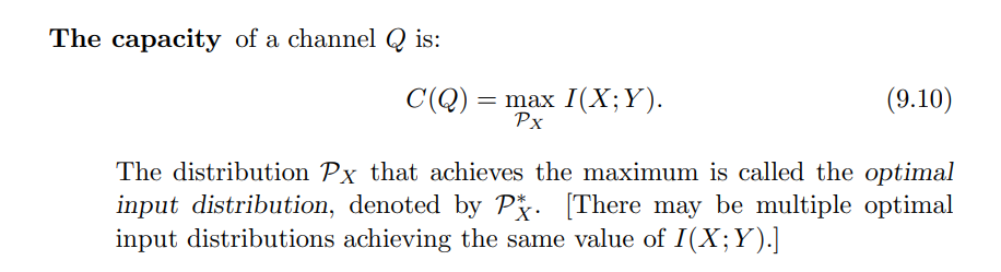
Channel Capacity
簡單一句話,channel capacity 就是改變 source distribution 得到最大的 mutual information.
$C = \max_X I(X;Y)$
-
$p(x,y) = p(y x) p(x)$, $p(y x)$ 是 transition (error) probability matrix. Transition probability matrix 不含 $X$ distribution。無法只用 transition probability matrix 得到 channel capacity. 不過如果是 symmetric channel, 一般 $p(x)$ 是 uniform distribution, 可以變成 normalization constant. Transition probability matrix 可以得到 channel capacity. -
Mutual Information $I(X;Y) = H(X) - H(X Y)$ 直接和 $X$ 的 distribution 相關。
Q: Why mutual information I(x;y) represents sending bits over the noisy channel?
A: Non-confusable subset: $2^{n I(X;Y)}$, normalize to unit time = $\frac{\log_2 2^{nI(X;Y)}}{n} = I(X;Y)$
實例和證明的構思
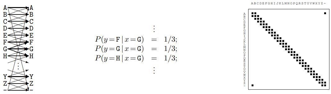
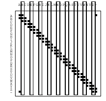
Example 1: Noisy typewriter channel
N = 1, Ax = Ay = {A, B, .., Z, -} 就是 26 個字母加上 - 號,凑成 27 個 symbol. 所謂的 noisy typewriter channel 就是每個字母都有 1/3 機會變成相鄰的字母或正確的字母,如下圖。
因爲 channel 是對所有字母對稱,似乎很合理假設 channel 最大的 capacity 是 uniform distribution?
Uniform Distribution of 27 字母
-
Transition probability 如上圖中: 1/3 or 0.
-
Joint probability 如上圖右, X 軸是 input symbol, Y 軸是 output symbol.
-
$P(X=A, Y=A) = P(Y=A X=A) P(X=A) = 1/3 \times 1/27$ -
$P(X=A, Y=B) = P(Y=B X=A) P(X=A) = 1/3 \times 1/27$ -
$P(X=A, Y=C) = P(Y=C X=A) P(X=A) = 0 \times 1/27 = 0$ -
$P(X, Y) = P(Y X) P(X) $, 因爲 P(X) 是 uniform distribution, $P(X,Y) = P(Y X) / 27$. [ 1/3/27 1/3/27 0 0 , … 1/3/27
1/3/27 1/3/27 1/3/27]
-
-
$H(X) = \log_2 27$, 同時 $H(Y) = \log_2 27$
- $H(X,Y) = \sum \frac{1}{3\times 27} \log_2 (3\times 27) = \log_2 (3\times27)$
- 其實如果是 uniform probability with $N$ points, $H = \log_2 N$
-
$I(X;Y) = H(X) + H(Y) - H(X,Y) = \log_2 27 + \log_2 27 - \log_2 (3\times 27) = \log_2 9$!
-
$H(Y X) = H(X,Y) - H(X) = \log_2 (3\times 27) - \log_2 27 = \log_2 3$ - It make sense! Given $x$, 對應 3 個 $y$ with equal probability (1/3,1/3,1/3), conditional entropy = $\log_2 3$
-
$H(X Y) = H(X,Y) - H(Y) = \log_2(3\times 27) - \log_2 27 = \log_2 3$ - It make sense! Given $y$, 對應 3 個 $x$ with equal probability (1/3,1/3,1/3), conditional entropy = $\log_2 3$
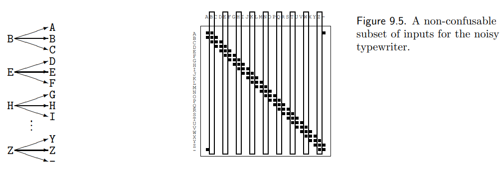
Non-confusable Subset (Uniform over 9 字母,非 27 字母)
如何能達到 arbitrary small error in this channel near channel capacity log_2(9)?
在這個 noisy channel 恰好非常容易!完全不用 error correction code! 而且一個 symbol 就可以完成。
我們先忘記 information theory, 用最簡單的幾何方法來解:
Error-free decode:
x 軸有 27 symbols, y 軸有 27 symbols. 一共有 3 x 27 點 (i.e. 每一點的機率是 1/(3*27), 不過不重要).
最簡單的 error-free communication 不是重複傳多次 (AAA, or AAAAA), 因爲這只是降低 error 的機率,無法保證 error free. 同時效率也不好。
比較好的方法是直接限制 transmit symbol, 讓 error 也被限制在一個範圍内。當然現實好像無法限制 error 只在前後一個字母,但讓我們假設可以辦到。
| 我們希望 p(x | y) = 1 or 0 (只有一個為 1). 這樣是 error-free. or H(X | Y) = 0, given Y, X 就沒有任何不確定性。 |
| 很明顯中間帶的寬度是 3 x 27 點 / 27 symbol = 3. 再來就是 input symbol 27 除以寬度 3 = 9! 所以限制 input 9 個 symbol 就可以達到 error free transmission. H(X) = log2(9) 因爲 H(X | Y) = 0. 所以 channel capacity = log2(9). |
考慮變形 case 1:
假如 input/output 有 27 symbol, 但是error 到鄰近 4 個 symbol.
點數 27 x 4 點 ( p(x,y) = 1/27/4 for x,y neq 0, 所以 H(X,Y) = log2(4*27), 點數= 2^log2(4**27) = 4 x 27)
| Y 寬度就會是 27 * 4 點數 / 27 Y symbol = 4 = (2^log2(4 27)/2^log2(27)). 此時就要限制 input 27/4 = 6.75 symbol. H(X) = H(X | Y) = log2(6.75) channel capacity 變小, make sense! |
Case 2: input output 不同 symbols, 例如 erasure channel
input 27, output 54, 點數 54 (等機率). 54/54 = 1, then 27/1 = 27 就是 information.
| point $2^{H(X,Y)}$, 寬度 $2^{H(X,Y)/2^{H(Y)}} = 2^{H(X | Y)}$ |
| Information = $2^{H(X)} / 2^{H(X | Y)} = 2^{(H(X)-H(X | Y))}= 2^{I(X;Y)}$!! |
H(x) = log_2(9)
H(y) = log_2(27)
- X has 9 值, Y 27 值
-
P(X=A, Y=A) = P(Y=A X=A) P(X=A) = 1/3 * 1/9 = P(X = A Y=A) P(Y=A) = 1 * 1/27 -
P(X=A, Y=B) = P(Y=B X=A) P(X=A) = 1/3 * 1/9 = P(X = A Y=B) P(Y=B) = 1 * 1/27 -
P(X=A, Y=C) = P(Y=C X=A) P(X=A) = 0 = P(X = A Y=C) P(Y=B) = 0
-
- H(x,y) = sum 1/27 * log_2(27) = log_2(27)
- I(x;y) = log_2(9) + log_2(27) - log_2(27) = log_2(9)!!
-
H(x y ) = H(x,y) - H(y) = log_2(27) - log_2(27) = 0!! H(Y X) = H(X,y) - H(x) = log_2(27) - log_2(9) = log_2(3) 都很 make sense! given Y, X 只有一個 value, 所以 entropy = 0; give X, Y 有三個 value, 所以 entropy = log_2(3)
Example 2: BSC Capacity
再回到 BSC 例子。因為是 symmetric channel, uniform distribution 對應最大 channel capacity.
$H_2(X) = 1, H_2(Y) = 1$ 因為 $X$ and $Y$ 都是 uniform distribution: Entropy = $\log_2 2 = 1$.
| $p(x,y) = p(y | x) p(x) = (1-p) * 0.5$ 當 $x=y$ |
| $p(x,y) = p(y | x) p(x) = p * 0.5$ 當 $x \ne y$ |
$H(X,Y) = -0.5(1-p) \log_2(0.5(1-p))\times 2 - 0.5 p \log_2(0.5p)\times 2$
$= -(1-p)\log_2(0.5(1-p)) - p \log_2(0.5p) = 1 - (1-p) \log_2 (1-p) - p \log_2 p$
$= 1 + H_2(p)$
$C = \max I(X;Y) = H(X) + H(Y) - H(X,Y) = 2 - 1 - H_2(p) = 1 - H_2(p)$
或是
| $C = H(X) - H(X | Y) = 1 - ( p \log_2 (1/p) + (1-p) \log_2 (1/(1-p))) = 1 + p \log_2(p) + (1-p) \log_2(1-p))$ |
| Make sense: (i) if X, Y independent, $H(X | Y) = H(X) \to C = 0$; (ii) if X, Y totally dependent, $H(X | Y) = 0 \to C = H(X)$. |
| Given Y, X 就是 biased coin with probability p, $H(X | Y) = H_2(p) \to C = 1 - H_2(p)$, 如下圖。 |
- p = 0.15 , C = 0.39 bit
- p = 0 or 1, C = 1-bit
- p = 0.5, C = 0-bit

最重要的問題:如何在 R < C = 0.39-bit 達到 error free communication?
造出 Non-Confusable Subset
Shannon 天才之處:
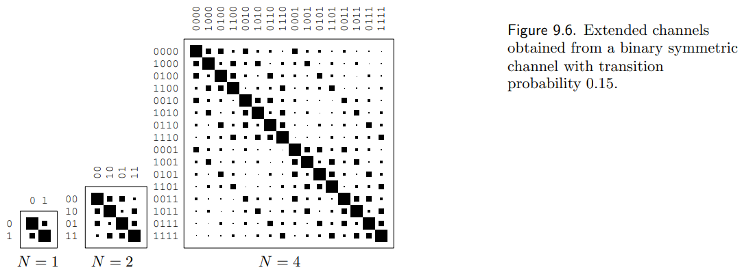
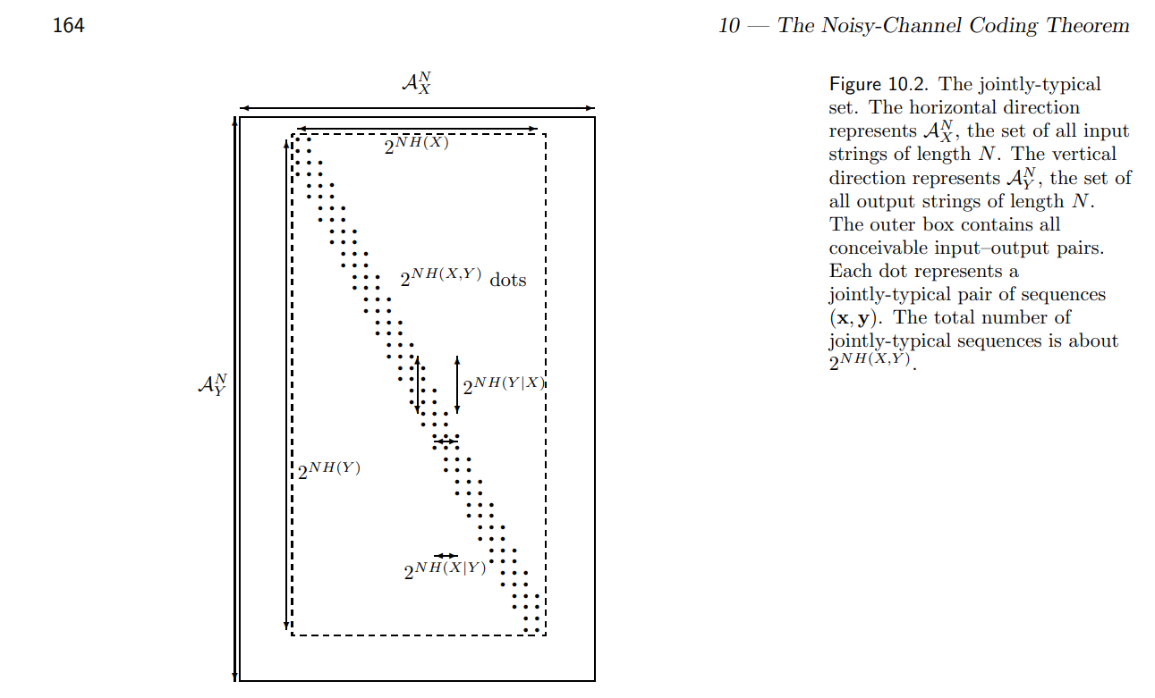
第一步: make N 很大 ($\mathcal{A}_X^N \times \mathcal{A}_Y^N$ box)!看起來很像 noisy typewriter!!! 問題是非中間帶不爲 0. 即使 N 到無窮大也不爲 0.
第二步: 雖然不爲 0, 但是可以任意小?中間帶可以定義 jointly typical? 基本 yes, 但是如何定義 jointly typical subset?
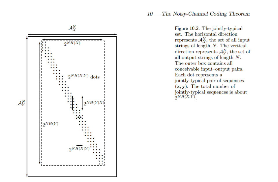
如下圖,要經過兩步加工!
(1) 證明所有 typical sets 都是在一個 inner box 中 ($2^{NH(X)} \times 2^{NH(Y)}$ ), 在 inner box 之外的機率可以任意小。
(2) 證明即使在 inner box 中,非 jointly-typical set 之外的機率可以任意小!
結論就如 noisy typewriter case:
平均而言: x,y 軸是 $2^{NH(X)} \times 2^{NH(Y)}$ , 對應 noisy typewriter 3 x 27.
有 significant 機率的 “dots” 基本有相等的機率 (統計力學的 equal partition theorem) 一共有 $2^{NH(X,Y)}$, 對應 noisy typewriter 3 x 27 dots, 每一點的幾率就是 1/ (3x27).
所以最後的 error free communication:
| noisy typewriter: H(Y) - H(Y | X) = log2(27) - log2(3) = log2(9) |
| this case: $NH(Y) - NH(Y | X) = N I(X;Y)$ 所以 /N => I(X;Y) |
| this case: $2^{NH(Y)} / 2^{NH(Y | X)} = 2^{NH(Y)-H(Y | X)} = 2^{N I(X;Y)}$ 所以 /N => I(X;Y) |
Typical Set and AEP Principle (參考 Appendix)
Jointly-typical set 如下:
| Input $X^n$ 的 typical set: $A^n_X$, and $ | A_X^n | = 2^{n H(X)}$ |
| Output $Y^n$ 的 typical set: $A^n_Y$, and $ | A_Y^n | = 2^{n H(Y)}$ |
| ($X^n, Y^n$) 的 typical set: $A_{XY}^n$, and $ | A_{XY}^n | = 2^{n H(X,Y)}$ |
關鍵:$N\to\infty$ Jointly-Typical Set $\to$ Non-confusable Subset
| **Why joint typical: $\log_2 P(X^n, Y^n) / n \sim H(X, Y)$? where $H(X, Y) = H(X) + H(Y | X) = H(Y) + H(X | Y)$** |
| 假設 BSC (Binary Symmetric Channel): $P(Y \ne X | X) = p, P(Y=X | X) = 1-p$ with $p = 0.2$ and $X, Y \in {H:0, T:1}$ |
EX1: $P(X=0) = P(X=1) = 0.5$. 因為是 symmetric channel, $P(Y=0)=P(Y=1)=0.5$
| 重點是 $P(X,Y)=P(Y | X)P(X)$, 如下表 |
| P(X=0) | P(X=1) | P(Y) | |
|---|---|---|---|
| P(Y=0) | P(Y|X) P(X) = 0.8 * 0.5 = 0.4 | P(Y|X) P(X) = 0.2 * 0.5 = 0.1 | 0.5 |
| P(Y=1) | P(Y|X) P(X) = 0.2 * 0.5 = 0.1 | P(Y|X) P(X) = 0.8 * 0.5 = 0.4 | 0.5 |
| P(X) | 0.5 | 0.5 | 1 |
- As a reference: $H(X) = H(Y) = H_2(0.5) = 1$-bit. $H(X, Y) = 1.722$-bit. $I(X;Y) = 0.278$-bit
Typical Set Example 1: N = 100 P(X=0 or 1) = 0.5, but transition probability = 0.2
$A_X^{100} = \underbrace{1 … 1}{50’s\, 1}\underbrace{0…0}{50’s\,0} \Rightarrow$ X typical sequence
$A_Y^{100} = \underbrace{1 … 1}{50’s\, 1}\underbrace{0…0}{50’s\,0} \Rightarrow$ Y typical sequence
| $P(Y=0 | X=0) = P(Y=1 | X=1) = 1$ and $P(Y=1 | X=0) = P(Y=0 | X=1) = 0$ |
所以 ${A_X^{100}, A_Y^{100}}$ 不是 (X, Y) jointly typical sequence!
Typical Set Example 2: n = 100 P(X=0 or 1) = 0.5, H(X)=H(Y)=1, but transition probability = 0.2
$A_X^{100} = \underbrace{1 … 1}{50’s\, 1}\underbrace{0…0}{50’s\,0} \Rightarrow$ P(X=0 or 1)=0.5, X typical sequence, 共有 $C(100,50) \approx 2^{nH(X)} = 2^{100} = 1.27\times 10^{30}$ sequences
$A_Y^{100} = \underbrace{1 … 1}{40’s\, 1}\underbrace{0…0}{10’s\,0} \underbrace{1 … 1}{10’s\, 1}\underbrace{0…0}{40’s\,0}\Rightarrow$ P(Y=0 or 1)=0.5, Y typical sequence, 共有 $C(100,50) \approx 2^{nH(Y)} = 2^{100} = 1.27\times 10^{30}$ sequences
| $P(Y=0 | X=0) = P(Y=1 | X=1) = 40/50 = 0.8$ and $P(Y=1 | X=0) = P(Y=0 | X=1) = 10/50 = 0.2$ |
所以 ${A_X^{100}, A_Y^{100}}$ 是 (X, Y) jointly typical sequence! 一共有多少 sequences?
-
Given X typical sequence, 50’s 1 以及 50’s 0, 把 20% 的 0 變成 1, 以及 1 變成 0.
-
$50!/(40! 10!) \times 50!/(40! 10!) = C(50,10) \times C(50,10) $
$= 2^{50 H(10/50)}\times 2^{50 H(10/50)} = 2^{100 H(0.2)} = 2^{72.2} = 5.42\times 10^{21}$.
-
但是 X 本身有 $2^{nH(X)}$ sequences, 所以 jointly sequences = $2^{nH(X)} 2^{100 H(0.2)} = 2^{100 (H(X)+H(0.2))} = 2^{100\times 1.722} = 2^{172.2} = 2^{n H(X,Y)}$
EX2: P(X=0 (H)) = 0.2, 因為非 symmetric channel, P(Y=0) = 0.32
重點是 P(x,y) 如下表
| P(X=0) | P(X=1) | P(Y) | |
|---|---|---|---|
| P(Y=0) | P(Y|X) P(X) = 0.8 * 0.2 = 0.16 | P(Y|X) P(X) = 0.2 * 0.8 = 0.16 | 0.32 |
| P(Y=1) | P(Y|X) P(X) = 0.2 * 0.2 = 0.04 | P(Y|X) P(X) = 0.8 * 0.8 = 0.64 | 0.68 |
| P(X) | 0.2 | 0.8 | 1 |
Example of Typical Set: N = 100 P(X=0 or 1) = 0.5
X = 11111,11111,11111,11111,00000,00000,0…0 (20 個 1,80 個 0). => X typical sequence
Y = 11111,11111,11111,11111,00000,00000,0…0 (20 個 1,80 個 0) => Y typical sequence
但是 X != (XOR) Y = 000..0 (100 個 0) => 非 jointly typical sequence, NOT (X,Y) jointly typical sequence
X = 11111,11111,11111,11111,00000,00000,0…0 (20 個 1,80 個 0). => X typical sequence
Y = 11111,11111,00000,00000,11111,11111,0… 0 (20 個 1,80 個 0) => Y typical sequence
X != (XOR) Y = 00000,00000,11111,11111,11111,11111,0… 0
| P(Y=1 | X=1) = 10/20 = 0.5; P(Y=0 | X=1) = 10/20 = 0.5 |
| P(Y=0 | X=0) = 70/80 = 0.875; P(Y=1 | X=0) = 10/80 = 0.125 |
(80 個 0, 10 個 1 (0->1), 10 個 1 (1->0) ) => Yes. (X,Y) jointly typical sequence
Appendix
Jointly Typical Definition
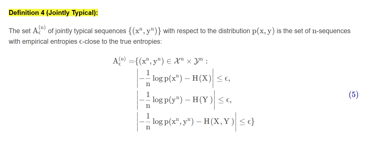
The set $A_{\varepsilon}^{n}$ of jointly typical sequences ${(X^n, Y^n)}$ with respect to the distribution $p(x,y)$ is the set of n-sequences with empirical entropies $\epsilon$-close to the true entropies:
\[\begin{aligned} A_\varepsilon^{n} = \left\{(X^{n}, {Y}^{n})\in \mathcal{X}^{n} \times \mathcal{Y}^{n} : \left|-\frac{1}{n} \log p\left(x^n\right)-H(X)\right| \leq \varepsilon, \right.\\ \left.\left|-\frac{1}{n} \log p\left(y^n\right)-H(Y)\right| \leq \varepsilon,\, \left|-\frac{1}{n} \log p\left(x^n, y^n\right)-H(X, Y)\right| \leq \varepsilon\right\} \end{aligned}\]這個式子有點長,不容易看懂!我之前一直糾結為什麼只有一個 $x^n$ 可以滿足不等式。
- Caveat: $p(x^n), p(y^n), p(x^n, y^n)$ 中的 $x^n, y^n$ 是所有滿足不等式的 sequences. 所有這些 sequences 的集合組成 jointly typical sequences!
Compression Typical Set Vs. Communication Typical Set
前文 information compression 的 typical set 定義比較清楚。只有第一段 $X$ 部分:$A_n^{\varepsilon}$ 的定義如下:
\[A^n_{\varepsilon}=\left\{\left(x_1, \cdots, x_n\right):\left|-\frac{1}{n} \log p\left(x_1, \cdots, x_n\right)-H(X)\right|<\varepsilon\right\} .\]可以看出 jointly typical set 的第一段和第二段其實和之前 typical set 定義完全一樣。
比較容易混淆是第三段 joint probability 和 joint entropy 的部分。我們再進一步澄清。
錯誤類比圖解
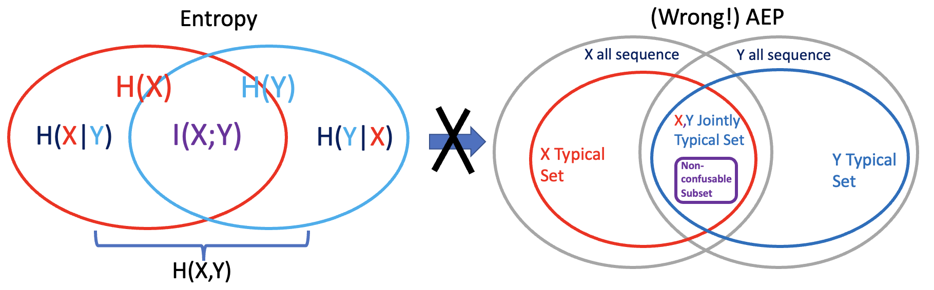
一個常見的錯誤是用 Joint Entropy 類比 Jointly typical set.
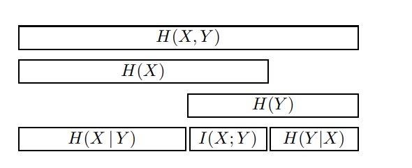
下圖左是 joint entropy 的示意圖,這是正確的。下圖右是錯誤的類比!X,Y jointly typical set 變成 X typical set 和 Y typical set 的交集, wrong!
交集表示 {X,Y jointly typical set} < {X typical set} 或是 {Y typical set}, Wrong!
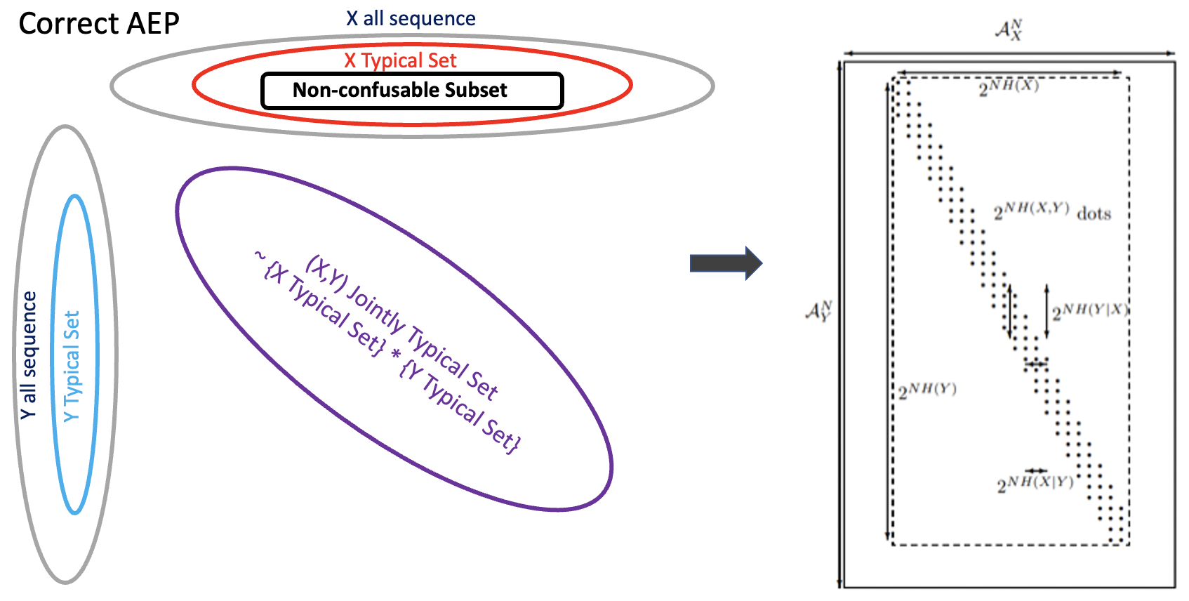
正確圖解
X, Y jointly typical set 比較類似 X typical set 和 Y typical set 的 “product” 而不是交集!如下圖。
Product 表示 {X,Y jointly typical set} > {X typical set} 或是 {Y typical set}
但 jointly typical set 也不是 direct product, 我們看幾個例子:
- X, Y independent
-
Entropy: $H(X, Y) = H(X) + H(Y); \quad H(Y X)=H(Y); \quad I(X; Y) = 0$ -
Typical set: $ A^n_X = 2^{n H(X)}; A^n_Y = 2^{n H(Y)}; A^n_{XY} = 2^{n H(X)} 2^{n H(Y)} = 2^{n (H(X)+H(Y))} = 2^{n H(X,Y)}$ -
$ A_{XY}^n = A_{X}^n A_{Y}^n $ : 這個 case, jointly typical set 是 direct product of X typical set and Y typical set. - Case 1: 下圖矩陣每個元素都不為 0,而且有同樣機率 (AEP)
- X, Y 完全 dependent (i.e. no noise)
-
Entropy: $H(X, Y) = H(X) = H(Y); \quad H(Y X) = 0 \quad I(X;Y) = H(X)$ -
Typical set: $ A^n_X = 2^{n H(X)} = A^n_Y = 2^{n H(Y)}; A^n_{XY} = 2^{n H(X)} = 2^{n H(X,Y)}$ -
$ A_{XY}^n = A_{X}^n = A_{Y}^n $ - Case 2: 下圖只有對角線的元素不為 0, 其他都是 0. 對角線的元素有相同的機率 (AEP).
- X, Y 部分 dependent (noisy channel)
-
Entropy: $H(X, Y) = H(X) + H(Y X) = H(X) + H(Y) - I(X; Y)$ -
Typical set: $ A^n_X = 2^{n H(X)}; A^n_Y = 2^{n H(Y)}$ -
Jointly typical set: $ A^n_{XY} = 2^{n H(X)} 2^{n H(Y X)} = 2^{n H(X, Y)}$ -
Jointly typical set 為什麼是 $2^{n H(X)} 2^{n H(Y X)}$? 因為 given 每一條 $X^n$ sequence, 都對應有 $2^{n H(Y X)}$ 條 $Y^n$ sequences. -
Case 3: 下圖對角線 band 的元素不為 0, 其他都是 0. 對角線的高度是 $2^{nH(Y X)}$, 所以所有非 0 元素才會是: $2^{n H(X)} 2^{n H(Y X)} = 2^{n H(X,Y)}$. 同樣對角線的寬度是 $2^{n H(X Y)}$. -
Non-confusable subset 就是:$2^{nH(X)}/2^{nH(X Y)}=2^{n(H(X)-H(X Y))}=2^{n I(X;Y)}$
AEP Theorem
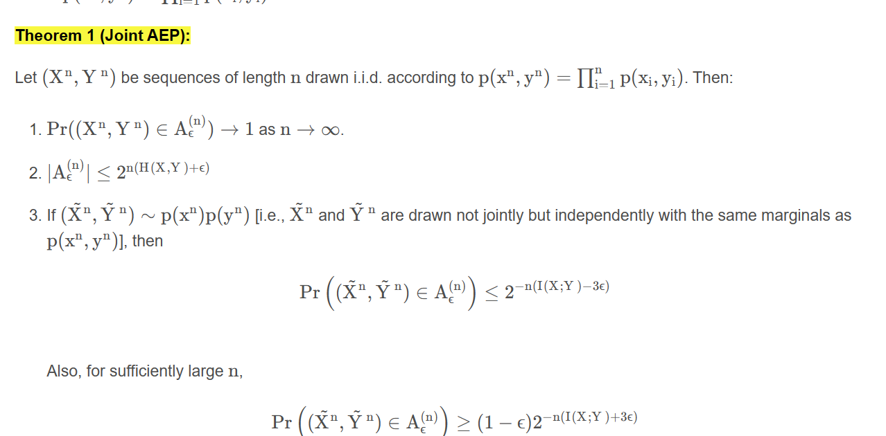
Let $\left(\mathrm{X}^{\mathrm{n}}, \mathrm{Y}^{\mathrm{n}}\right)$ be sequences of length $\mathrm{n}$ drawn i.i.d. according to $\mathrm{p}\left(\mathrm{x}^{\mathrm{n}}, \mathrm{y}^{\mathrm{n}}\right)=\prod_{\mathrm{i}=1}^{\mathrm{n}} \mathrm{p}\left(\mathrm{x}{\mathrm{i}}, \mathrm{y}{\mathrm{i}}\right)$. Then:
- $\operatorname{Pr}\left(\left(\mathrm{X}^{\mathrm{n}}, \mathrm{Y}^{\mathrm{n}}\right) \in \mathrm{A}_\epsilon^{(\mathrm{n})}\right) \rightarrow 1$ as $\mathrm{n} \rightarrow \infty$.
-
$\left \mathrm{A}_\epsilon^{(\mathrm{n})}\right \leq 2^{\mathrm{n}(\mathrm{H}(\mathrm{X}, \mathrm{Y})+\epsilon)}$ - If $\left(\tilde{\mathrm{X}}^{\mathrm{n}}, \tilde{\mathrm{Y}}^{\mathrm{n}}\right) \sim \mathrm{p}\left(\mathrm{x}^{\mathrm{n}}\right) \mathrm{p}\left(\mathrm{y}^{\mathrm{n}}\right)$ [i.e., $\tilde{\mathrm{X}}^{\mathrm{n}}$ and $\tilde{\mathrm{Y}}^{\mathrm{n}}$ are drawn not jointly but independently with the same marginals as $\left.\mathrm{p}\left(\mathrm{x}^{\mathrm{n}}, \mathrm{y}^{\mathrm{n}}\right)\right]$, then \(\operatorname{Pr}\left(\left(\tilde{\mathrm{X}}^{\mathrm{n}}, \tilde{\mathrm{Y}}^{\mathrm{n}}\right) \in \mathrm{A}_\epsilon^{(\mathrm{n})}\right) \leq 2^{-\mathrm{n}(\mathrm{I}(\mathrm{X} ; \mathrm{Y})-3 \epsilon)}\)
Also, for sufficiently large $\mathrm{n}$, \(\operatorname{Pr}\left(\left(\tilde{\mathrm{X}}^{\mathrm{n}}, \tilde{\mathrm{Y}}^{\mathrm{n}}\right) \in \mathrm{A}_\epsilon^{(\mathrm{n})}\right) \geq(1-\epsilon) 2^{-\mathrm{n}(\mathrm{I}(\mathrm{X} ; \mathrm{Y})+3 \epsilon)}\)
I(X; Y) depends on X distribution and channel. The capacity of a channel 是找到最好的 X distribution to maximize I(X;Y)
Old Material, to be deleted
Information Theory of Dependent Random Variable (Chap 8)