Download the code: https://github.com/allenlu2009/colab/blob/master/dataframe_demo.ipynb
Python DataFrame
Create DataFrame
-
Direct input
-
Use dict: Method 1: 一筆一筆加入。
1 | |
| Name | Sex | Age | |
|---|---|---|---|
| 0 | Allen | male | 33 |
| 1 | Alice | female | 22 |
| 2 | Bob | male | 11 |
Method 2: 一次加入所有資料。
1 | |
| Name | Age | |
|---|---|---|
| 0 | Allen | 33 |
| 1 | Alice | 22 |
| 2 | Bob | 11 |
Dataframe 的屬性
- ndim: 2 for 2D dataframe; axis 0 => row; axis 1 => column
- shape: (row no. x column no.) (not including number index)
- dtypes: (object or int) of each column
1 |
|
1 |
|
1 |
|
1 | |
1 |
|
1 | |
1 | |
1 | |
1 |
|
1 | |
Read CSV
Donwload a test csv file from https://people.sc.fsu.edu/~jburkardt/data/csv/csv.html Pick the biostats.csv
For 2, Before read csv, reference Medium article to import google drive
- Read csv 使用 read_csv function. 但是要加上 skipinitialspace to strip the leading space!!
- Two ways to read_csv: (1) load csv file directly; (2) load from url
1 | |
1 | |
| Name | Sex | Age | Height (in) | Weight (lbs) | |
|---|---|---|---|---|---|
| 0 | Alex | M | 41 | 74 | 170 |
| 1 | Bert | M | 42 | 68 | 166 |
| 2 | Carl | M | 32 | 70 | 155 |
| 3 | Dave | M | 39 | 72 | 167 |
| 4 | Elly | F | 30 | 66 | 124 |
| 5 | Fran | F | 33 | 66 | 115 |
| 6 | Gwen | F | 26 | 64 | 121 |
| 7 | Hank | M | 30 | 71 | 158 |
| 8 | Ivan | M | 53 | 72 | 175 |
| 9 | Jake | M | 32 | 69 | 143 |
| 10 | Kate | F | 47 | 69 | 139 |
| 11 | Luke | M | 34 | 72 | 163 |
| 12 | Myra | F | 23 | 62 | 98 |
| 13 | Neil | M | 36 | 75 | 160 |
| 14 | Omar | M | 38 | 70 | 145 |
| 15 | Page | F | 31 | 67 | 135 |
| 16 | Quin | M | 29 | 71 | 176 |
| 17 | Ruth | F | 28 | 65 | 131 |
1 | |
1 | |
1 |
|
1 |
|
1 |
|
1 |
|
1 |
|
1 | |
Basic Viewing Command
1 | |
| Name | Sex | Age | Height (in) | Weight (lbs) | |
|---|---|---|---|---|---|
| 0 | Alex | M | 41 | 74 | 170 |
| 1 | Bert | M | 42 | 68 | 166 |
| 2 | Carl | M | 32 | 70 | 155 |
1 | |
| Name | Sex | Age | Height (in) | Weight (lbs) | |
|---|---|---|---|---|---|
| 15 | Page | F | 31 | 67 | 135 |
| 16 | Quin | M | 29 | 71 | 176 |
| 17 | Ruth | F | 28 | 65 | 131 |
1 |
|
1 |
|
1 | |
1 | |
1 | |
| Name | Sex | Age | Height (in) | Weight (lbs) | |
|---|---|---|---|---|---|
| 7 | Hank | M | 30 | 71 | 158 |
| 8 | Ivan | M | 53 | 72 | 175 |
| 9 | Jake | M | 32 | 69 | 143 |
1 | |
1 | |
1 | |
| Name | Age | Sex | |
|---|---|---|---|
| 7 | Hank | 30 | M |
| 8 | Ivan | 53 | M |
| 9 | Jake | 32 | M |
1 | |
| Name | Age | Sex | |
|---|---|---|---|
| 7 | Hank | 30 | M |
| 8 | Ivan | 53 | M |
| 9 | Jake | 32 | M |
| 10 | Kate | 47 | F |
1 | |
1 | |
Basic Index Operation
Index (索引) is a very useful key for DataFrame. The default index is the row number starting from 0 to N-1, where N is the number of data. 除了用 row number 做為 index, 一般也會使用 unique feature 例如 name, id, or phone number 做為 index.
把 column 變成 index
- Method 1: 直接在 read_csv 指定 index_col. 可以看到 index number 消失,而被 Name column 取代。
1 | |
| Sex | Age | Height (in) | Weight (lbs) | |
|---|---|---|---|---|
| Name | ||||
| Alex | M | 41 | 74 | 170 |
| Bert | M | 42 | 68 | 166 |
| Carl | M | 32 | 70 | 155 |
| Dave | M | 39 | 72 | 167 |
| Elly | F | 30 | 66 | 124 |
| Fran | F | 33 | 66 | 115 |
| Gwen | F | 26 | 64 | 121 |
| Hank | M | 30 | 71 | 158 |
| Ivan | M | 53 | 72 | 175 |
| Jake | M | 32 | 69 | 143 |
| Kate | F | 47 | 69 | 139 |
| Luke | M | 34 | 72 | 163 |
| Myra | F | 23 | 62 | 98 |
| Neil | M | 36 | 75 | 160 |
| Omar | M | 38 | 70 | 145 |
| Page | F | 31 | 67 | 135 |
| Quin | M | 29 | 71 | 176 |
| Ruth | F | 28 | 65 | 131 |
- df.index shows the element in index column
1 |
|
1 | |
- 使用 reset_index 又會回到 index number.
1 |
|
| Name | Sex | Age | Height (in) | Weight (lbs) | |
|---|---|---|---|---|---|
| 0 | Alex | M | 41 | 74 | 170 |
| 1 | Bert | M | 42 | 68 | 166 |
| 2 | Carl | M | 32 | 70 | 155 |
| 3 | Dave | M | 39 | 72 | 167 |
| 4 | Elly | F | 30 | 66 | 124 |
| 5 | Fran | F | 33 | 66 | 115 |
| 6 | Gwen | F | 26 | 64 | 121 |
| 7 | Hank | M | 30 | 71 | 158 |
| 8 | Ivan | M | 53 | 72 | 175 |
| 9 | Jake | M | 32 | 69 | 143 |
| 10 | Kate | F | 47 | 69 | 139 |
| 11 | Luke | M | 34 | 72 | 163 |
| 12 | Myra | F | 23 | 62 | 98 |
| 13 | Neil | M | 36 | 75 | 160 |
| 14 | Omar | M | 38 | 70 | 145 |
| 15 | Page | F | 31 | 67 | 135 |
| 16 | Quin | M | 29 | 71 | 176 |
| 17 | Ruth | F | 28 | 65 | 131 |
再看一次 df 並沒有改變。很多 DataFrame 的 function 都是保留原始的 df, create a new object, 也就是 inplace = False. 如果要取代原來的 df, 必須 inplace = True!
1 |
|
| Sex | Age | Height (in) | Weight (lbs) | |
|---|---|---|---|---|
| Name | ||||
| Alex | M | 41 | 74 | 170 |
| Bert | M | 42 | 68 | 166 |
| Carl | M | 32 | 70 | 155 |
| Dave | M | 39 | 72 | 167 |
| Elly | F | 30 | 66 | 124 |
| Fran | F | 33 | 66 | 115 |
| Gwen | F | 26 | 64 | 121 |
| Hank | M | 30 | 71 | 158 |
| Ivan | M | 53 | 72 | 175 |
| Jake | M | 32 | 69 | 143 |
| Kate | F | 47 | 69 | 139 |
| Luke | M | 34 | 72 | 163 |
| Myra | F | 23 | 62 | 98 |
| Neil | M | 36 | 75 | 160 |
| Omar | M | 38 | 70 | 145 |
| Page | F | 31 | 67 | 135 |
| Quin | M | 29 | 71 | 176 |
| Ruth | F | 28 | 65 | 131 |
1 | |
| Name | Sex | Age | Height (in) | Weight (lbs) | |
|---|---|---|---|---|---|
| 0 | Alex | M | 41 | 74 | 170 |
| 1 | Bert | M | 42 | 68 | 166 |
| 2 | Carl | M | 32 | 70 | 155 |
| 3 | Dave | M | 39 | 72 | 167 |
| 4 | Elly | F | 30 | 66 | 124 |
| 5 | Fran | F | 33 | 66 | 115 |
| 6 | Gwen | F | 26 | 64 | 121 |
| 7 | Hank | M | 30 | 71 | 158 |
| 8 | Ivan | M | 53 | 72 | 175 |
| 9 | Jake | M | 32 | 69 | 143 |
| 10 | Kate | F | 47 | 69 | 139 |
| 11 | Luke | M | 34 | 72 | 163 |
| 12 | Myra | F | 23 | 62 | 98 |
| 13 | Neil | M | 36 | 75 | 160 |
| 14 | Omar | M | 38 | 70 | 145 |
| 15 | Page | F | 31 | 67 | 135 |
| 16 | Quin | M | 29 | 71 | 176 |
| 17 | Ruth | F | 28 | 65 | 131 |
如果再 reset_index()一次,會是什麼結果?此處用 default inplace=False. 多了一個 index column
1 |
|
| index | Name | Sex | Age | Height (in) | Weight (lbs) | |
|---|---|---|---|---|---|---|
| 0 | 0 | Alex | M | 41 | 74 | 170 |
| 1 | 1 | Bert | M | 42 | 68 | 166 |
| 2 | 2 | Carl | M | 32 | 70 | 155 |
| 3 | 3 | Dave | M | 39 | 72 | 167 |
| 4 | 4 | Elly | F | 30 | 66 | 124 |
| 5 | 5 | Fran | F | 33 | 66 | 115 |
| 6 | 6 | Gwen | F | 26 | 64 | 121 |
| 7 | 7 | Hank | M | 30 | 71 | 158 |
| 8 | 8 | Ivan | M | 53 | 72 | 175 |
| 9 | 9 | Jake | M | 32 | 69 | 143 |
| 10 | 10 | Kate | F | 47 | 69 | 139 |
| 11 | 11 | Luke | M | 34 | 72 | 163 |
| 12 | 12 | Myra | F | 23 | 62 | 98 |
| 13 | 13 | Neil | M | 36 | 75 | 160 |
| 14 | 14 | Omar | M | 38 | 70 | 145 |
| 15 | 15 | Page | F | 31 | 67 | 135 |
| 16 | 16 | Quin | M | 29 | 71 | 176 |
| 17 | 17 | Ruth | F | 28 | 65 | 131 |
1 |
|
| Name | Sex | Age | Height (in) | Weight (lbs) | |
|---|---|---|---|---|---|
| 0 | Alex | M | 41 | 74 | 170 |
| 1 | Bert | M | 42 | 68 | 166 |
| 2 | Carl | M | 32 | 70 | 155 |
| 3 | Dave | M | 39 | 72 | 167 |
| 4 | Elly | F | 30 | 66 | 124 |
| 5 | Fran | F | 33 | 66 | 115 |
| 6 | Gwen | F | 26 | 64 | 121 |
| 7 | Hank | M | 30 | 71 | 158 |
| 8 | Ivan | M | 53 | 72 | 175 |
| 9 | Jake | M | 32 | 69 | 143 |
| 10 | Kate | F | 47 | 69 | 139 |
| 11 | Luke | M | 34 | 72 | 163 |
| 12 | Myra | F | 23 | 62 | 98 |
| 13 | Neil | M | 36 | 75 | 160 |
| 14 | Omar | M | 38 | 70 | 145 |
| 15 | Page | F | 31 | 67 | 135 |
| 16 | Quin | M | 29 | 71 | 176 |
| 17 | Ruth | F | 28 | 65 | 131 |
- Method 2: 使用 set_index()
1 | |
| Sex | Age | Height (in) | Weight (lbs) | |
|---|---|---|---|---|
| Name | ||||
| Alex | M | 41 | 74 | 170 |
| Bert | M | 42 | 68 | 166 |
| Carl | M | 32 | 70 | 155 |
| Dave | M | 39 | 72 | 167 |
| Elly | F | 30 | 66 | 124 |
| Fran | F | 33 | 66 | 115 |
| Gwen | F | 26 | 64 | 121 |
| Hank | M | 30 | 71 | 158 |
| Ivan | M | 53 | 72 | 175 |
| Jake | M | 32 | 69 | 143 |
| Kate | F | 47 | 69 | 139 |
| Luke | M | 34 | 72 | 163 |
| Myra | F | 23 | 62 | 98 |
| Neil | M | 36 | 75 | 160 |
| Omar | M | 38 | 70 | 145 |
| Page | F | 31 | 67 | 135 |
| Quin | M | 29 | 71 | 176 |
| Ruth | F | 28 | 65 | 131 |
loc[]
使用 loc[] 配合 index label 取出資料非常方便。
如果是 number index, 可以用 df[0], df[3], etc.
但如果是其他 column index, e.g. Name, df[2] 或是 df[“Hank”] are wrong!, 必須用 df.loc[‘Hank’]
或是 df.loc[ [‘Hank’, ‘Ruth’, ‘Page’] ]
1 | |
1 | |
1 | |
| Sex | Age | |
|---|---|---|
| Name | ||
| Alex | M | 41 |
| Bert | M | 42 |
| Carl | M | 32 |
| Dave | M | 39 |
| Elly | F | 30 |
| Fran | F | 33 |
| Gwen | F | 26 |
| Hank | M | 30 |
| Ivan | M | 53 |
| Jake | M | 32 |
| Kate | F | 47 |
| Luke | M | 34 |
| Myra | F | 23 |
| Neil | M | 36 |
| Omar | M | 38 |
| Page | F | 31 |
| Quin | M | 29 |
| Ruth | F | 28 |
1 | |
| Sex | Age | Height (in) | Weight (lbs) | |
|---|---|---|---|---|
| Name | ||||
| Hank | M | 30 | 71 | 158 |
| Ruth | F | 28 | 65 | 131 |
| Page | F | 31 | 67 | 135 |
loc[] 可以用 row, column 得到對應的 element, 似乎是奇怪的用法
1 | |
1 | |
iloc[]
使用 column index 仍然可以用 iloc[] 配合 index number 取出資料。
1 | |
1 | |
1 | |
| Sex | Age | Height (in) | Weight (lbs) | |
|---|---|---|---|---|
| Name | ||||
| Bert | M | 42 | 68 | 166 |
| Carl | M | 32 | 70 | 155 |
| Dave | M | 39 | 72 | 167 |
| Elly | F | 30 | 66 | 124 |
| Fran | F | 33 | 66 | 115 |
| Gwen | F | 26 | 64 | 121 |
| Hank | M | 30 | 71 | 158 |
| Ivan | M | 53 | 72 | 175 |
| Jake | M | 32 | 69 | 143 |
1 | |
| Sex | Age | Height (in) | Weight (lbs) | |
|---|---|---|---|---|
| Name | ||||
| Bert | M | 42 | 68 | 166 |
| Elly | F | 30 | 66 | 124 |
| Gwen | F | 26 | 64 | 121 |
排序
包含兩種排序
- sort_index()
- sort_value()
1 | |
| Sex | Age | Height (in) | Weight (lbs) | |
|---|---|---|---|---|
| Name | ||||
| Alex | M | 41 | 74 | 170 |
| Bert | M | 42 | 68 | 166 |
| Carl | M | 32 | 70 | 155 |
| Dave | M | 39 | 72 | 167 |
| Elly | F | 30 | 66 | 124 |
| Fran | F | 33 | 66 | 115 |
| Gwen | F | 26 | 64 | 121 |
| Hank | M | 30 | 71 | 158 |
| Ivan | M | 53 | 72 | 175 |
| Jake | M | 32 | 69 | 143 |
| Kate | F | 47 | 69 | 139 |
| Luke | M | 34 | 72 | 163 |
| Myra | F | 23 | 62 | 98 |
| Neil | M | 36 | 75 | 160 |
| Omar | M | 38 | 70 | 145 |
| Page | F | 31 | 67 | 135 |
| Quin | M | 29 | 71 | 176 |
| Ruth | F | 28 | 65 | 131 |
1 | |
| Sex | Age | Height (in) | Weight (lbs) | |
|---|---|---|---|---|
| Name | ||||
| Myra | F | 23 | 62 | 98 |
| Gwen | F | 26 | 64 | 121 |
| Ruth | F | 28 | 65 | 131 |
| Quin | M | 29 | 71 | 176 |
| Elly | F | 30 | 66 | 124 |
| Hank | M | 30 | 71 | 158 |
| Page | F | 31 | 67 | 135 |
| Carl | M | 32 | 70 | 155 |
| Jake | M | 32 | 69 | 143 |
| Fran | F | 33 | 66 | 115 |
| Luke | M | 34 | 72 | 163 |
| Neil | M | 36 | 75 | 160 |
| Omar | M | 38 | 70 | 145 |
| Dave | M | 39 | 72 | 167 |
| Alex | M | 41 | 74 | 170 |
| Bert | M | 42 | 68 | 166 |
| Kate | F | 47 | 69 | 139 |
| Ivan | M | 53 | 72 | 175 |
Rename and Drop Column(s) and Index(s)
1 | |
| Sex | Age | Height | Weight | |
|---|---|---|---|---|
| Name | ||||
| Alex | M | 41 | 74 | 170 |
| Bert | M | 42 | 68 | 166 |
| Carl | M | 32 | 70 | 155 |
| Dave | M | 39 | 72 | 167 |
| Elly | F | 30 | 66 | 124 |
| Fran | F | 33 | 66 | 115 |
| Gwen | F | 26 | 64 | 121 |
| Hank | M | 30 | 71 | 158 |
| Ivan | M | 53 | 72 | 175 |
| Jake | M | 32 | 69 | 143 |
| Kate | F | 47 | 69 | 139 |
| Luke | M | 34 | 72 | 163 |
| Myra | F | 23 | 62 | 98 |
| Neil | M | 36 | 75 | 160 |
| Omar | M | 38 | 70 | 145 |
| Page | F | 31 | 67 | 135 |
| Quin | M | 29 | 71 | 176 |
| Ruth | F | 28 | 65 | 131 |
1 | |
| Sex | Age | Height | Weight | |
|---|---|---|---|---|
| Name | ||||
| Allen | M | 41 | 74 | 170 |
| Bob | M | 42 | 68 | 166 |
| Carl | M | 32 | 70 | 155 |
| Dave | M | 39 | 72 | 167 |
| Elly | F | 30 | 66 | 124 |
| Fran | F | 33 | 66 | 115 |
| Gwen | F | 26 | 64 | 121 |
| Hank | M | 30 | 71 | 158 |
| Ivan | M | 53 | 72 | 175 |
| Jake | M | 32 | 69 | 143 |
| Kate | F | 47 | 69 | 139 |
| Luke | M | 34 | 72 | 163 |
| Myra | F | 23 | 62 | 98 |
| Neil | M | 36 | 75 | 160 |
| Omar | M | 38 | 70 | 145 |
| Page | F | 31 | 67 | 135 |
| Quin | M | 29 | 71 | 176 |
| Ruth | F | 28 | 65 | 131 |
1 | |
| Age | Height | |
|---|---|---|
| Name | ||
| Allen | 41 | 74 |
| Bob | 42 | 68 |
| Carl | 32 | 70 |
| Dave | 39 | 72 |
| Elly | 30 | 66 |
| Fran | 33 | 66 |
| Gwen | 26 | 64 |
| Hank | 30 | 71 |
| Ivan | 53 | 72 |
| Jake | 32 | 69 |
| Kate | 47 | 69 |
| Luke | 34 | 72 |
| Myra | 23 | 62 |
| Neil | 36 | 75 |
| Omar | 38 | 70 |
| Page | 31 | 67 |
| Quin | 29 | 71 |
| Ruth | 28 | 65 |
1 | |
| Sex | Age | Height | Weight | |
|---|---|---|---|---|
| Name | ||||
| Bob | M | 42 | 68 | 166 |
| Carl | M | 32 | 70 | 155 |
| Dave | M | 39 | 72 | 167 |
| Elly | F | 30 | 66 | 124 |
| Fran | F | 33 | 66 | 115 |
| Gwen | F | 26 | 64 | 121 |
| Hank | M | 30 | 71 | 158 |
| Ivan | M | 53 | 72 | 175 |
| Jake | M | 32 | 69 | 143 |
| Kate | F | 47 | 69 | 139 |
| Luke | M | 34 | 72 | 163 |
| Myra | F | 23 | 62 | 98 |
| Neil | M | 36 | 75 | 160 |
| Omar | M | 38 | 70 | 145 |
| Page | F | 31 | 67 | 135 |
| Quin | M | 29 | 71 | 176 |
進階技巧
Multiple Index (多重索引)
這是非常有用的技巧,使用 set_index with keys
1 | |
| Name | Sex | Age | Height (in) | Weight (lbs) | |
|---|---|---|---|---|---|
| 0 | Alex | M | 41 | 74 | 170 |
| 1 | Bert | M | 42 | 68 | 166 |
| 2 | Carl | M | 32 | 70 | 155 |
| 3 | Dave | M | 39 | 72 | 167 |
| 4 | Elly | F | 30 | 66 | 124 |
| 5 | Fran | F | 33 | 66 | 115 |
| 6 | Gwen | F | 26 | 64 | 121 |
| 7 | Hank | M | 30 | 71 | 158 |
| 8 | Ivan | M | 53 | 72 | 175 |
| 9 | Jake | M | 32 | 69 | 143 |
| 10 | Kate | F | 47 | 69 | 139 |
| 11 | Luke | M | 34 | 72 | 163 |
| 12 | Myra | F | 23 | 62 | 98 |
| 13 | Neil | M | 36 | 75 | 160 |
| 14 | Omar | M | 38 | 70 | 145 |
| 15 | Page | F | 31 | 67 | 135 |
| 16 | Quin | M | 29 | 71 | 176 |
| 17 | Ruth | F | 28 | 65 | 131 |
1 | |
| Age | Height (in) | Weight (lbs) | ||
|---|---|---|---|---|
| Name | Sex | |||
| Alex | M | 41 | 74 | 170 |
| Bert | M | 42 | 68 | 166 |
| Carl | M | 32 | 70 | 155 |
| Dave | M | 39 | 72 | 167 |
| Elly | F | 30 | 66 | 124 |
| Fran | F | 33 | 66 | 115 |
| Gwen | F | 26 | 64 | 121 |
| Hank | M | 30 | 71 | 158 |
| Ivan | M | 53 | 72 | 175 |
| Jake | M | 32 | 69 | 143 |
| Kate | F | 47 | 69 | 139 |
| Luke | M | 34 | 72 | 163 |
| Myra | F | 23 | 62 | 98 |
| Neil | M | 36 | 75 | 160 |
| Omar | M | 38 | 70 | 145 |
| Page | F | 31 | 67 | 135 |
| Quin | M | 29 | 71 | 176 |
| Ruth | F | 28 | 65 | 131 |
1 | |
| Age | Height (in) | Weight (lbs) | ||
|---|---|---|---|---|
| Sex | Name | |||
| M | Alex | 41 | 74 | 170 |
| Bert | 42 | 68 | 166 | |
| Carl | 32 | 70 | 155 | |
| Dave | 39 | 72 | 167 | |
| F | Elly | 30 | 66 | 124 |
| Fran | 33 | 66 | 115 | |
| Gwen | 26 | 64 | 121 | |
| M | Hank | 30 | 71 | 158 |
| Ivan | 53 | 72 | 175 | |
| Jake | 32 | 69 | 143 | |
| F | Kate | 47 | 69 | 139 |
| M | Luke | 34 | 72 | 163 |
| F | Myra | 23 | 62 | 98 |
| M | Neil | 36 | 75 | 160 |
| Omar | 38 | 70 | 145 | |
| F | Page | 31 | 67 | 135 |
| M | Quin | 29 | 71 | 176 |
| F | Ruth | 28 | 65 | 131 |
1 |
|
1 | |
1 | |
1 | |
1 | |
1 | |
1 | |
| Age | Height (in) | Weight (lbs) | ||
|---|---|---|---|---|
| Sex | Name | |||
| F | Elly | 30 | 66 | 124 |
| Fran | 33 | 66 | 115 | |
| Gwen | 26 | 64 | 121 | |
| Kate | 47 | 69 | 139 | |
| Myra | 23 | 62 | 98 | |
| Page | 31 | 67 | 135 | |
| Ruth | 28 | 65 | 131 | |
| M | Alex | 41 | 74 | 170 |
| Bert | 42 | 68 | 166 | |
| Carl | 32 | 70 | 155 | |
| Dave | 39 | 72 | 167 | |
| Hank | 30 | 71 | 158 | |
| Ivan | 53 | 72 | 175 | |
| Jake | 32 | 69 | 143 | |
| Luke | 34 | 72 | 163 | |
| Neil | 36 | 75 | 160 | |
| Omar | 38 | 70 | 145 | |
| Quin | 29 | 71 | 176 |
Groupby Command
Groupby 是 SQL 的語法。根據某一項資料做分組方便查找。
The SQL GROUP BY Statement
The GROUP BY statement is often used with aggregate functions (COUNT, MAX, MIN, SUM, AVG) to group the result-set by one or more columns.
1 | |
| Sex | Age | Height (in) | Weight (lbs) | |
|---|---|---|---|---|
| Name | ||||
| Alex | M | 41 | 74 | 170 |
| Bert | M | 42 | 68 | 166 |
| Carl | M | 32 | 70 | 155 |
| Dave | M | 39 | 72 | 167 |
| Elly | F | 30 | 66 | 124 |
| Fran | F | 33 | 66 | 115 |
| Gwen | F | 26 | 64 | 121 |
| Hank | M | 30 | 71 | 158 |
| Ivan | M | 53 | 72 | 175 |
| Jake | M | 32 | 69 | 143 |
| Kate | F | 47 | 69 | 139 |
| Luke | M | 34 | 72 | 163 |
| Myra | F | 23 | 62 | 98 |
| Neil | M | 36 | 75 | 160 |
| Omar | M | 38 | 70 | 145 |
| Page | F | 31 | 67 | 135 |
| Quin | M | 29 | 71 | 176 |
| Ruth | F | 28 | 65 | 131 |
1 | |
1 | |
1 | |
1 | |
1 | |
1 | |
1 | |
| Sex | Age | Height (in) | Weight (lbs) | |
|---|---|---|---|---|
| Name | ||||
| Alex | M | 41 | 74 | 170 |
| Bert | M | 42 | 68 | 166 |
| Carl | M | 32 | 70 | 155 |
| Dave | M | 39 | 72 | 167 |
| Hank | M | 30 | 71 | 158 |
| Ivan | M | 53 | 72 | 175 |
| Jake | M | 32 | 69 | 143 |
| Luke | M | 34 | 72 | 163 |
| Neil | M | 36 | 75 | 160 |
| Omar | M | 38 | 70 | 145 |
| Quin | M | 29 | 71 | 176 |
Groupby Operation
分組後可以進行各類運算:sum(), mean(), max(), min()
1 | |
| Age | Height (in) | Weight (lbs) | |
|---|---|---|---|
| Sex | |||
| F | 218 | 459 | 863 |
| M | 406 | 784 | 1778 |
1 | |
| Age | Height (in) | Weight (lbs) | |
|---|---|---|---|
| Sex | |||
| F | 31.142857 | 65.571429 | 123.285714 |
| M | 36.909091 | 71.272727 | 161.636364 |
1 | |
| Age | Height (in) | Weight (lbs) | |
|---|---|---|---|
| Sex | |||
| F | 47 | 69 | 139 |
| M | 53 | 75 | 176 |
1 | |
| Age | Height (in) | Weight (lbs) | |
|---|---|---|---|
| Sex | |||
| F | 23 | 62 | 98 |
| M | 29 | 68 | 143 |
Wash Data with NAN
判斷 NAN
- isnull()
- notnull()
處理 NAN
- dropna()
- fillna()
1 | |
1 | |
Plot
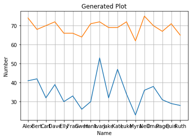
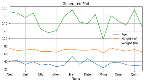
DataFrame 一個很重要的特性是利用 matplotlib.pyplot 繪圖功能 visuallize data!
有兩種方式:(1) 直接用 df.plot; (2) 用 pyplot 的 plot.
(1) 是一個 quick way to plot
(2) 可以調用 pyplot 所有的功能
1 | |
1 | |
1 | |