AI-NR (as virtual lighting!) use visual effect to see how many dB gain by AI-NR!
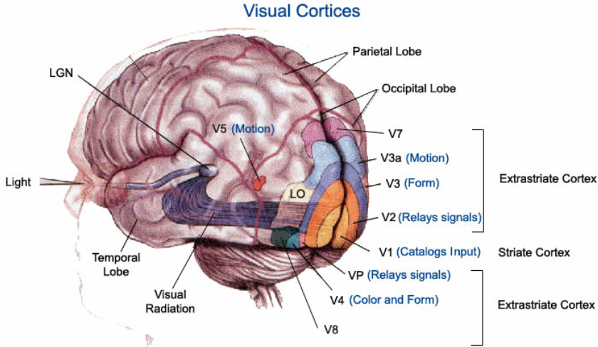
在討論 computer vision 之前,先看人類視覺:包含眼睛和大腦。當小美看到小明時,眼睛的視網膜把光信號轉換成電信號;其中桿狀細胞對於亮度 (luma) 敏感,錐狀細胞對於顔色 (chroma) 敏感。視神經傳導電信號先經過 LGN (位於丘腦, thalamus) 中繼站,再傳送到枕葉 (occipital lobe) 的視覺皮質,這大約耗時 10’s ms. 視覺處理的第一站是 V1, 稱爲 primary visual cortex, 皮質區域和視網膜視野基本一一對應。V1的功能依照屬性分類顏色、方向、空間、位置,將訊息傳至其他 VX 和相關部位。
主要有兩條路線:一是判別空間的背側路徑 (dorsal stream 或稱爲 where or how pathway),例如空間、方向、顔色 (V4)、motion (V3/V3a/V5)。另一個是識別該物體的腹側路線 (ventral stream 或稱爲 what or who pathway),人臉辨識 (FFA)、物體辨識走的就是這條路徑。
V1-V5 非常簡化的功能如下:
- V1 功能:立體視覺 (i.e. depth estimation), 物體位置、方向、大小、形狀等基本功能。
- V2 功能:表達 (represent) 和識別 (recognize) 物體,和大腦的記憶部位 (e.g. 海馬回) 溝通 via ventral stream.
- V4 功能:顔色。
- V3/V3a/V5 ( V5 也稱爲 MT):Motion 包含方向和速度。
- Fusiform Face Area (FFA, not shown):Face detection and recognition
Why discuss human vision?
- Leverage the knowledge of human vision for major computer vision tasks and classification. What can or cannot be done.
- Take advantage of human vision strength or weakness. How to please human vision (HDR, SR, MEMC, etc.) or how to cheat human vision to trade-off processing and power (e.g. VRS, )
Wiki 對於 computer vision 的定義如下:
簡單的概念就是可以用數學表達是最重要的 base. CV 算法一般指可以用數學定性和定量描述。對應 NN 算法一般深度學習網絡,需要用 大量 data training 得到的 weights, 也就是目前常常説的 AI 算法。 相性之下,比較 black box.
| CV algorithm | NN algorithm (AI) | |
|---|---|---|
| Application | Vision | Vision, Voice/Speech, NLP, Robotics |
| Math | Many different forms, mostly math clearly explained | Deep neural network |
| Data | few or no need | big data learning |
| ML | Shallow ML is part of CV algorithm | Part of ML |
| Example | HOG, SIFT | ResNet, |
| Future direction | CV (as prior) + NN | General, CV+NN, interpretable, |
A good reference from Nancy Kanwisher of MIT OCW course about Neuroscience
And Marr’s computation theory, representation theory?
我的邏輯 (OP -> CV or NN -> visual perception)
類比與人腦對於 vision 的做法,結合物理數學定律。把 vision 分解成基本的 building block,提出一一對應招式 (operation or op)。其實這就是 analyze - to dissect, take to pieces 的意義。這也是從一個學長得到的靈感。
第一層的分解:Space (3D) and Time (1D) - 符合牛頓的時空觀。這裏就對不起愛因斯坦的時空觀,因爲人腦的確是在遠低於光速的演化,也最適合于牛頓的時空觀。這也是爲什麽人腦對於愛因斯坦的時空觀覺得怪異 (e.g. 長度收縮,時間膨脹,不同慣性坐標系時間不同步)。不是不理解,而是”不直觀”。
把 4D 分解成 3D (space) + 1D (time) 很重要,一個是把問題簡單化。另外也是讓計算複雜度降低,才能 enable 不同的應用。我們之後會從應用面演進趨勢來看:voice (1D time) -> photo (2D plane) -> video (2D plane+1D time) -> VR/AR (3D space + 1D time) ,剛好相反。就是 follow 計算能力增加的結果。
Static and Spatial (靜態空間):例如 2D or 3D 照片
這裏包含 2D 的照片,全景 (360) 照片,3D stereoscope image,or 3D hologram.
我們再分一層:2D (plane) and 3D (space)
2D stationary 基本視覺感知 visual perception: resolution/edge/detail, color/brightness/contrast
2D Resolution
-
2D vision 最基本重要的 op 就是改變 resolution, 包含 resolution up and resolution down. 主要是爲了讓 image or video from camera or network 能夠顯示在各種尺寸大小的 display (e.g. TV, PC/Laptop, tablet, smartphone). 舉例而言 YouTube video 大多是 720p (1280x720 pixel) 或是 1080p (1920x1080 pixel),當要顯示在 4K TV (3840x2160 pixel) 就需要增加 resolution, 或是 pixel 的數目。相反現在很多手機和 camera 可以拍攝 4K 或是更高解析度的 photo or video, 當要顯示在 1080p screen, 需要降低 resolution.
-
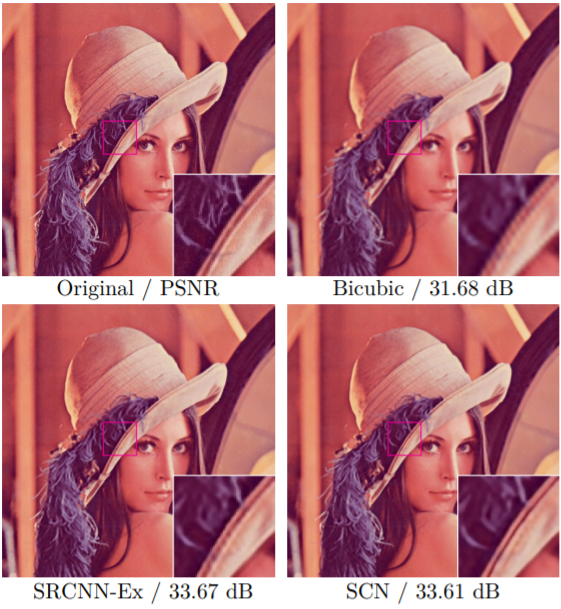
注意改變 resolution 不只是簡單的幾何放大 (e.g. add nearest neighbor pixel) 或縮小 (e.g. delete pixel),還需要保留對 visual perception 有意義的細節 (e.g. edge)。對應的 CV (computer vision) 算法包含 bilinear, bicubical, lancos; 對應的 NN (neural network) 算法包含各種 super resolution, 如下圖除了 original, 其他如 Bicubic (CV) , SRCNN (NN), SCN (NN) 都放大 3X in length, or 9x in area.
-
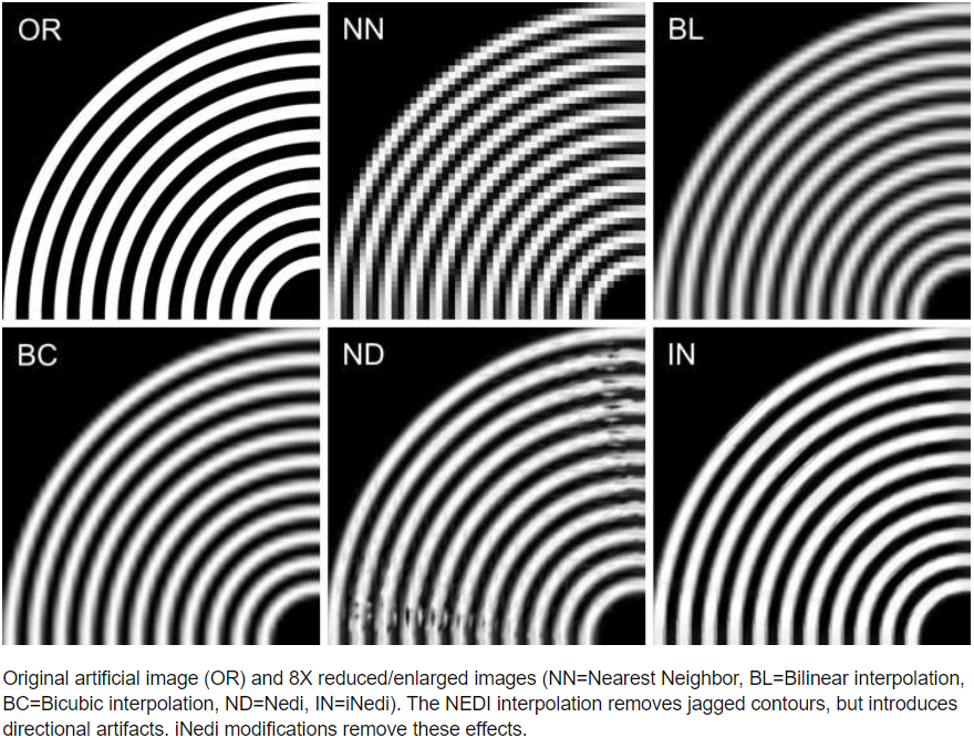
人腦對於人造物體 (e.g. 建築綫條,文字) 的 edge 特別敏感,like jagged edge (x), blurry edge (x), thin line (x). 下圖左是 original (OR);圖中是 resize (8X resize) 使用 nearest neighbor (NN in this case, not Neural Network) 避免模糊,但卻造成 jagged edge;圖右是用 bilinear interpolation (BL) and the next one is bicubic interpolation (BC), 兩者都有 blurry edge.
-
Resolution 和 visual perception 的關聯,最終是由 visual perception 的 retina density (~400 dpi) 對應的 viewing angle (?) 決定。到底能不能看到一些 details.
Color depth/brightness/contrast 對應視覺的錐狀細胞 (顔色) 和柱狀細胞 (亮度)
- 2D vision 另一個重要 op 是 color depth/brightness/contrast. 在 low light (or under exposure, 曝光不足) 要提高 contrast,亮光時色彩 (color) 要鮮艷,强光時壓低 brightness. CV 對應的算法是 (global or local) tone adjustment for high dynamic range (HDR). 一般是 content indepdent. NN 的算法就是 SDR-to-HDR (e.g. HDRnet), 一般是 pixel-based and content dependent algorithm. Without surprise, NN 的算法比 CV 算法效果更好。
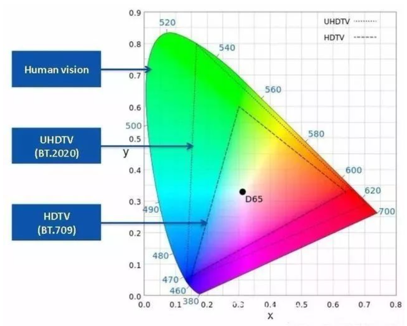
- Human vision 有非常大的 dynamic range, 如上圖所示。目前 TV display or smartphone display 的 dynamic range 都小於 human vision. 而 input image (photo or video) 的 dynamic range 可能遠小於 HDR display, 更不用說 human vision. 代表 color depth 的 limitation 是由 display 所決定。隨著 display 技術的進步,例如 mini-LED, OLED, or micro-LED, display 技術會愈來愈接近 human vision. 代表 SDR-to-HDR 還有很大的空間。
其他的 2D op 如 scale, translation, mirror, rotation. 不過這似乎比較是單純幾何數學運算 (assuming the same resolution),統稱爲 CV 算法。
2D Visual perception summary
- 自然界的東西大多是連續 and smooth (e.g. sky, grass, leaf); or context bland surface (如墻面) low pass filter
- 對於人造的建築,edge,綫條,剛好相反,LPF 會看起來模糊,要特別加强對比。(i.e. high frequency component)
- Lighting, low light 時人眼對於 color 不敏感。同時也比較模糊。相反在亮光時,色彩要比較鮮艷。强光的地方反而要壓低 gamma curve 避免 saturate.
再來就是比較高級或複雜的視覺感知,位於大腦區域而不是眼睛。傳統的 CV 算法, i.e. 數學公式, 已經無法處理,需要用 NN (i.e. AI) 算法才有比較滿意的結果。這也是 NN 大顯身手的開始。
高級的視覺感知 visual perception: segmentation, object localization, object classification, object detection 需要用 NN 算法。
從視覺感知而言,segmentation (物體和背景輪廓) 和 localization (物體位置,using bounding box or center point) 不涉及認知,是比較 primitive (但不意味比較簡單) 的功能。大多數會跑、會跳、會游的動物視覺都有這個功能。 Object classification 和 object detection 1 不只是感知,還有認知 (cognition) 的功能,一般是比較 “聰明” 的動物,如猩猩,海豚,當然還有人類具有的功能。
不過從 neural network 的角度,classification 似乎比較“簡單”,Segmentation (or localization) 反而比較“複雜”,原因可能
- Segmentation 是 pixel level 的 operation from input to output, end-to-end 是降維再升維過程,整體的計算量非常大,感覺複雜度更高。 Classification 雖然是 pixel level input, 但是 output 卻只是一個名稱 (label),end-to-end 是降維過程,整體的計算量比較小。
- Segmentation dataset 數目和大小比起 classification 少,而且 label 的準確度也比較差。這也可能讓 segmentation 的 SOTA 不如人類 (as far as I know). 但 classification 經過 ImageNet 多年的訓驗,SOTA 早就超過人類。
- 目前 segmentation 主流 NN model (e.g. DeepLab V3, UNet) 都是基於 CNN 變化得出。也許還有更適合的 network model for segmentation.
我們從 primitive 功能開始討論。
Image Segmentation (i.e. No Depth)
- Segmentation 是介於 pixel-level and object-level 的 operation, 簡單說就是找到物體在不同空間 (land, sky, background) 的邊界。這對於視覺非常重要。也充分體現視覺和聽覺不同的地方。簡單來説,視覺一般有清晰的邊界,除了在有烟、霧、雨特殊情況下例外。聽覺沒有清楚的邊界,除非用在超音波影像。從物理的角度,就是光波的波長遠小於日常生活物體,很難繞射;聲波的波長遠大約日常生活物體(除非是超音波),很難不繞射。視覺有 locality, occulusion, 等等的物質 (matter) 的性質,聽覺大多是加強,抵消,或混在一起接近波動 (wave) 的性質。 所以 image segmentation 可説是視覺獨有的 operation, 聽覺就沒有所謂的 segmentation.
- 相形之下,detection 和 classification 基本上都有視覺和聽覺的版本。
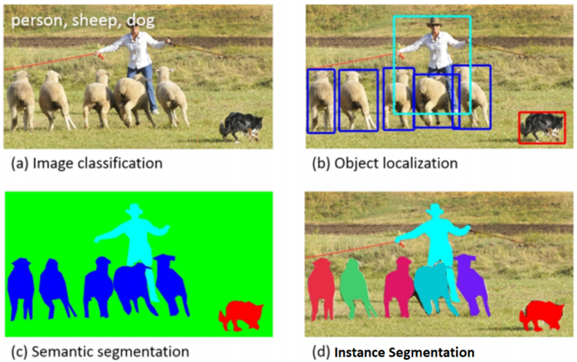
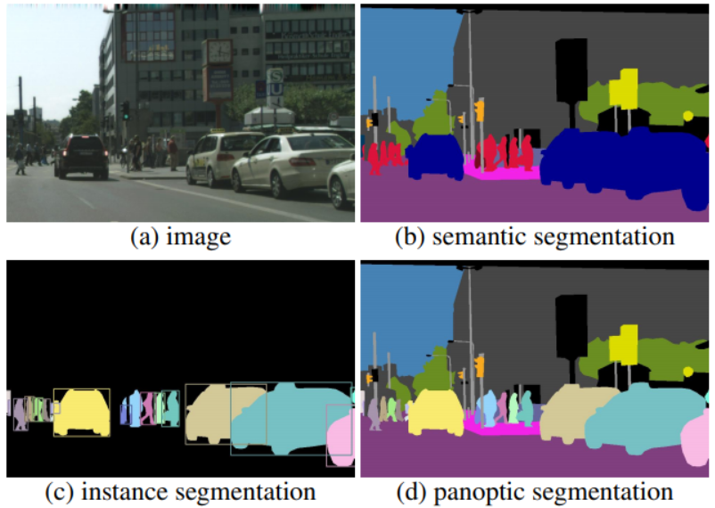
- 從數學的角度,就是要對 image 的每一個 pixel 做分類。基本上有三種不同階層的 image segmentation,如下圖 (b), (c), (d).
- 基本的是 semantic segmentation (b): “Both syntax and semantics are key parts in language but have unique linguistic meanings. Put simply, syntax refers to grammar, while semantics refers to meaning.” Semantic segmentation 顧名思義是 ”語義 (圖義) 分割”,這裏 semantics 是指同一類 (class) 物件 pixel 的集合,例如人是紅色,車是藍色,等等。但注意這裏的 semantics 並沒有物體的名稱 (e.g. 人,車),甚至沒有區分個別物體 (object or instace), 而是物體的集合。
- 進一步是 instance segmentation (c): 就是區分物件,不管背景。這裏 instance 是指同一個物件 pixel 的集合。同樣 instance segmentation 本身並沒有物體的名稱。實務上 instance segmentation 和 object detection 會用一個 NN (e.g. mask-RCNN), 同時得到物體的輪廓和名稱。
- Panoptic segmentation (d) = semantic segmentation + instance segmentation. 此處不再贅述。
Object Detection and Classification
首先 Object Detection = Object Localization (位置) + Object Classification (名稱)
從視覺的角度,localization 和 classification 是兩件事。Localization 只是感知物體的位置,要再經過認知 (cognition) 的 classification 才能判斷是 friend /foe/food.
一般是一個 NN 處理 classification, e.g. ResNet, MobileNet. 再用這個 NN 為 backbone 延伸得到位置 using bounding box or center point, e.g. SSD, YOLO. 這和視覺似乎相反?
先看 object classification = feature extraction + classification
Classification 可以再拆解成 feature extraction + classification 如下圖。傳統的 machine learning (ML) 是由人工來做 feature extraction, 再利用分類網絡 (e.g. Support Vector Machine, Softmax) 做 classification. Deep learning (DL), 或稱爲 NN, 利用 end-to-end training 自動學習出 feature extraction 和分類網絡,開啓了第三波 AI 的浪潮。
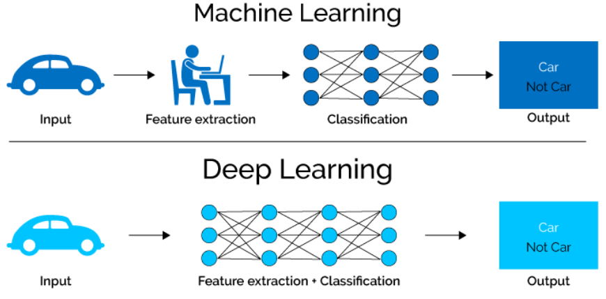
Feature extraction: 一般是假設 feature space (or manifold in 非歐空間) 維度遠小於 input image/video 維度。Feature extraction 是一個降維的 operation, CNN 已經證明是非常有效的 local feature extraction 工具,再加上 transformer 的 global attention 是目前的 SOTA network, 例如 ViT, Swin, etc.
Classification: 目前主流的 image feature classification 是 fully-connected layers + softmax network, 主要是: (1) 讓 classification network 單純,複雜的部分交給 feature extraction network; (2) 可以和 CNN 串接一起訓練。缺點是 FC+softmax 可調的參數很多,在 training dataset 不夠大時很容易 overfit. 另外參數多也佔 memory, 同時造成 memory bandwidth bottleneck.
除了 softmax, 在特定的應用也會使用不同的 classification function, 例如 angle classification in 人臉識別。
再來是 object localization (Position)
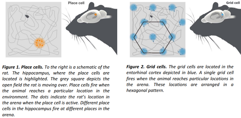
2014 諾貝爾生理獎得主發現哺乳動物 (e.g. 老鼠,人) 大腦的對於空間的定位和導航系統包含 place cell and grid cell, 非常有趣! [kiehnBrainNavigational2014]
- Place cell 位於海馬迴,簡單說是一種 landmark system, 類似相對位置。在看到熟悉的 landmark 就可以定位目前的位置, Fig. 1.
- Grid cell 位於內嗅皮層,非常靠近海馬迴。是一種是 grid system, 類似絕對位置和距離, Fig. 2.
- 據説女生比較依靠 place cell,男生比較依靠 grid cell. 所以女生喜歡逛 shopping mall or supermarket, 很快能找到要買的店或東西。男生擅長看地圖,根據方向和距離導航。
Object localization 只是在 2D (or 3D) 影像對於物體的定位,還用不到這麽複雜的空間定位和導航系統。主要是針對視覺内物體的位置和大小。但算法上似乎有類似的做法、
- Anchor or anchorless: anchor 類似相對位置? anchorless 類似絕對位置? or the other way around?
- Bounding box or center point + radius? Bounding 似乎比較 make sense 因爲除了給位置還給出大小。
In summary
| OP | CV | NN | Visual | Math/Physics | |
|---|---|---|---|---|---|
| 2D space | |||||
| Resolution/Edge/Detail | Resolution Up/Dn for display | interpolation | Pixel SR/UNet | Retina angle; how to please eyes? | equvariant |
| Color/Brightness/Contrast | SDR to HDR | tone map | Pixel HDR | Vision map; how to please eyes? | equvariant, RBGW; |
| Segmentation | Pixel UNet | equvariant | |||
| Feature Extraction | CNN+attention | invariant | |||
| Localization | Object xxx | equvariant | |||
| Classification | FC+Softmax | invariant |
3D to 2D Spatial Information Loss
真實世界的物體是 3D,只是投影到 display 甚至是 retina 都是 2D pixel。最後在大腦又重組回 3D perception.
最大的問題就是 3D to 2D 會造成 depth (深度) 的資訊丟失 (information loss) 如下圖。在缺乏深度資訊的情況下,不同形狀的 3D objects 在視網膜投影 2D 影像都一樣,造成 ambiguity. 因此從 2D retina image pixel 推論出 3D 空間 (voxel) 的 object 或 motion 一般很困難,這稱爲 ill-posed problem.

有幾類方法可以 reconstruct 3D 空間的 voxel (類比 2D 平面的 pixel): (1) direct 3D sensor; (2) depth map + 2D image; (3) multiple viewing angle + 2D images. 其中 (1) 和 (2) 可以直接用數學公式算出 3D voxel, 一般定義為 CV 算法。(3) 因爲 viewing angle 不限定,目前主流是用 deep learning (NN) 算法。
-
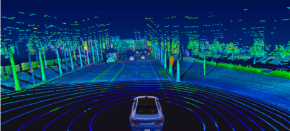
Direct 3D sensor 像是 Lidar, ToF (time of flight) 得到的 3D voxel 圖如下。後面可能再要接一個分類網絡判斷樹,車,人等等。
-
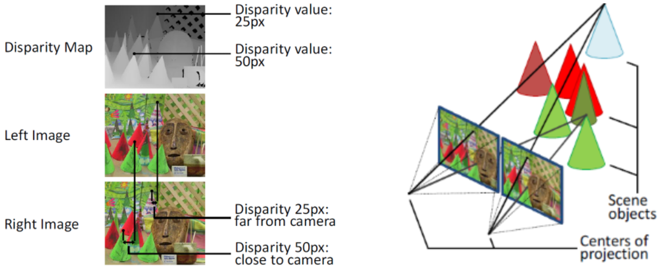
一般用 stereoscope (或者雙目視覺) 三角測量法得到 depth map 如下圖左。從 depth map + 2D image 可以得到 3D voxel 圖,如下圖右。另外在 graphics 或是 gaming 的應用中,object 的 depth 是已知的資訊, i.e. prior information. 因此在 gaming 可以很容易做 3D domain operation (e.g. 移動)
-
真正的挑戰是用一個 camera (monocular) 產生 depth map. 一般需要移動 camera viewing angle (e.g. video). 如果要同時,只能多個 cameras 的影像合成。Multiple viewing angle 乍看之下和雙目視覺相同 (兩個視角),實際上更複雜。雙目視覺一般有 well-defined and fixed viewing angle, i.e. same horizontal with a pre-defined separating distance, 如上圖。 Multiple viewing angle 則可能有任意的 viewing angle, either by moving the camera or moving the object (e.g. video). 具體的做法可以參考 review paper, 此處不討論。
Depth map 一般不是最後的目的,而是開始。從 depth map 可以 infer 更複雜的 3D 應用,例如立體視覺 (3D photo or hologram)、ray tracing, 3D object detection, 3D object tracking, 3D navigation. 這些複雜的 3D 應用大多需要利用 NN (i.e. AI) 算法。此時 NN 的 input 就會是 RGB+D (depth).
Temporal (動態):Motion
視覺另一個非常重要的維度是時間,對應的就是 motion,大腦 cortex 甚至有專門的區域 V5 (MT) 處理 motion, 包含方向和速度。
大腦可以處理單眼或雙眼的 motion. 一般單眼偵測的是 cast 到 2D 平面的 motion, 如前所述,因爲缺乏深度資訊,這是一個 ill-posed problem. 相反雙眼 (立體) 視覺, structure light, lidar 等則可以得出深度資訊 (2D 平面 motion + 1D 深度),或是直接偵測 3D 空間的移動。這就變成一個 well-defined 數學問題,可以用 CV 算法解決。
不過雖然是 ill-posed, 但并不是完全沒有機會
- 假如 motion 主要是 object 非深度方向的移動 (e.g. surveillance camera), 或是 camera 非深度方法的移動 (e.g. change viewing angle for panorama), 就不是那麽 ill-posed.
- object or camera 本身的移動也造成 viewing angle change, 間接提供深度的資訊。
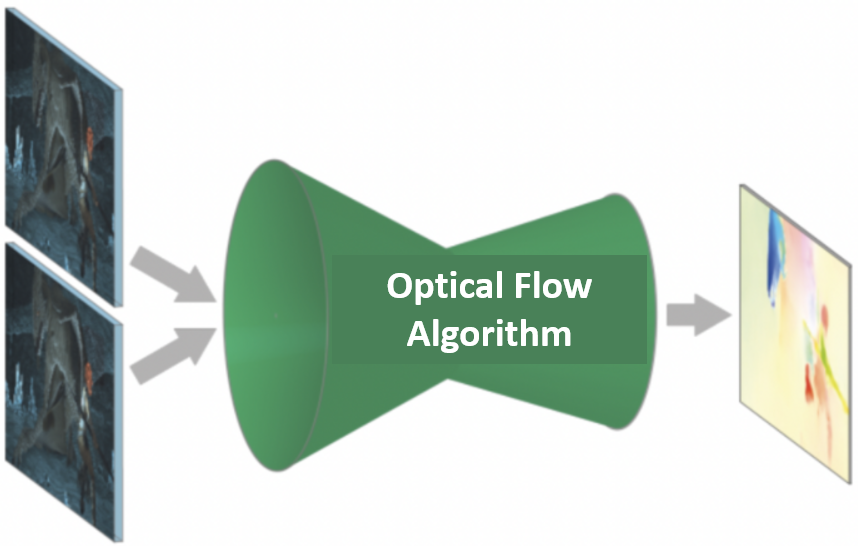
光流 (Optical Flow) 直觀解釋
如何偵測 2D 平面的 motion? 這就要介紹赫赫有名的光流 (optical flow). 乍聼之下好像是一個非常厲害的方法,其實 optical flow 非常簡單直觀,也是大腦判斷 motion 速度和方向的方式。
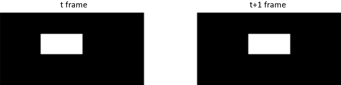
光流 in a nutshell:物體移動的方向就是光流動的方向!
這好像是一句廢話。但什麽是光流動的方向?直觀說物體移動方向就是物體變亮的方向,或是物體變暗的反方向。以下圖白色方形爲例,左圖是 T 時刻的位置,右圖是 T+1 時刻的位置。想像播放連續的 T, T+1, …, video frames, 物體的右邊持續變亮 (或是物體的左邊持續變暗)。大腦直覺的反應就是白色方形向右移動。大腦不用分析每一幀白色方形位置才得到這個正確的結論。這也代表大腦也是利用光流法判斷物體移動方向。
光流偏微分解釋 (CV 算法)
用數學來推導光流法:用同樣上圖的例子,但是假設白色到黑色有 smooth 的 transition w.r.t $x$, 如下圖上。 如何從 $I(x,t)\to I(x, t+\Delta t)$ 估計出移動速度 $v$? 基本和 $I(x,t)$ 對時間和空間的偏微分相關,數學的推導參考 appendix.

在一些假設下,可以得到一個簡單的公式:(1) constant illumination, i.e. dI(x,t)/dt = 0 (2). small motion.
我們用以下的 3D 圖給出物理的解釋。
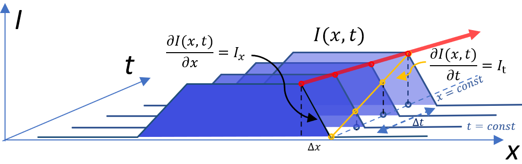
假設光向右邊流動,一個點 $x$ 包含附近 $\Delta x$, 的區域的亮度會隨空間變小 (上圖黑綫,斜率 $I_x$ at fixed $t$,就是 gradient),亮度則會隨時間 $\Delta t$ 變大 (上圖黃綫,斜率 $I_t$ at fixed $x$,對時間一階導數). 我們現在要解的是紅綫的斜率,i.e. $v = - \frac{\Delta x}{\Delta t}$ at a fixed $\Delta I$.
簡單來說,$x$ 點 local 的亮度變化 $\Delta I$ 可以是由於空間變化 $\Delta x = \frac{\Delta I}{I_x}$; 或是由於時間變化是 $\Delta t = \frac{\Delta I}{I_t}$. 假設 global 的亮度不會隨時間變大或變小,只是從 $(t_0, x_0) \to (t_1, x_1)$. 我們可以從同樣的亮度改變推論光流的速度,
\[v \approx - \frac{\Delta x}{\Delta t} = - \frac{\frac{\Delta I}{I_x}}{\frac{\Delta I}{I_t}} = - \frac{I_t}{I_x} \quad \text{assuming constant luminescent; small motion}\]where \(I_{x}=\left.\frac{\partial I}{\partial x}\right|_{t} \quad I_{t}=\left.\frac{\partial I}{\partial t}\right|_{x=p}\)
更數學一點的說明,假設我們要 trace 某一點 $x$ 的亮度變化 w.r.t space and time, i.e. $I(x, t)$. 同時 as an optical flow $x$ 是 function of $t$, i.e. $x(t)$.
\[\frac{d I}{d t} = \frac{\partial I}{\partial t} + \frac{\partial I}{\partial x} \frac{d x}{d t} = I_t + I_x V_x\]同樣假設我們要 trace 的是亮度不變的光流速度:$\frac{d I}{d t} = 0 \Rightarrow V_x = - \frac{I_t}{I_x}$ 這個結果和之前直覺得到的結果一致!
上式的好處是可以直接推廣到 2D 光流,這是實際真正有用的光流。順帶一提,如果推廣到 3D 就稱為 scene flow, 此處不討論。
2D Optical Flow Equation with constant luminescence assumption
\[\frac{d I}{d t} = \frac{\partial I}{\partial t} + \frac{\partial I}{\partial x} \frac{d x}{d t} + \frac{\partial I}{\partial y} \frac{d y}{d t}= I_t + I_x V_x + I_y V_y = I_t + \nabla I \cdot \vec{V} = 0\] \[I_{t} = - \nabla I \cdot \vec{V} = -(I_{x} V_{x}+I_{y} V_{y})\]幾個重點:
-
$I_x$ and $I_y$ 不能為全都為 0, 這樣任何的 $V_x$ and $V_y$ 都是 optical flow equation 的解。這很直觀,例如一部純白的車子在純白的背景移動,或是純黑的車子在黑夜移動,都無法判斷車子的速度。即使純白的車子在黑色的背景移動,如上上上圖,除了在邊界的地方可以判斷速度;在遠離邊界的地方因為沒有 gradient, 其實同樣是無法判斷速度。這些 gradient=0 的地方,都是 optical flow 的 ill-condition. 不過一般自然的 object motion (e.g. 人,動物) in image or video, 很少會有大片 gradient=0 的地方。就算有,一般也是背景 (e.g. 天空,道路,黑夜) 沒有 motion 的地方,比較沒有影響。
-
Optical flow 的 input 一般是兩張 image with $\Delta t$ 時間差,output 是 motion map (vector map), 例如下圖。
-
Optical flow 是偏微分方程,就像其他的偏微分方程 (e.g. fluid flow, heat flow),需要靠 boundary condition 才能確定真正的解。如果沒有 boundary condition, 就有可能造成另外的 ill-condition. 在 optical flow 有所謂的孔徑問題,見下圖,三個完全不同方向的運動孔徑内都會有同樣的 local pattern. 如果沒有其他的 boundary condition, 只看 local pattern, 無法唯一決定 optical flow 的方向。
-
大腦視覺也是利用 optical flow (and constant brightness 假設) 判斷 motion. 同樣會 suffer ill-condition. 例如下圖的理髮廳的旋轉招牌,也是利用孔徑問題。明明 motion 是水平移動,視覺卻是向上移動,因爲招牌的形狀暗示大腦是垂直運動。所以大腦會產生視覺錯覺或是空間迷向。斑馬也許是利用這個特性迷惑獵食者。順帶一提,當視覺方向和其他感官 (e.g. 耳内的平衡器官) 判斷方向不同時,就會造成暈眩和噁心。有一些遊樂設施就是利用這些特性挑戰游客。

-
偏微分方程一般歸類在 CV 算法。因為用 neural network, NN, 很難直接偏微分方程。常見的 optical flow CV 算法包含 L&K (Lucas, Kandade) 或 H&S (Horn, Schunck),分為對應 sparse optical flow 和 dense optical flow 算法。
Limitation of Optical Flow Based On CV Algorithm
-
Only small variation, otherwise H.O.T (high order term) is not negligble \(I(\mathbf{x}+\partial \mathbf{x}, t+\partial t)=I(\mathbf{x}, t)+\nabla I \cdot \mathbf{v}+\frac{\partial I}{\partial t}+H . O . T .\) where $\mathbf{v}=\frac{\partial \mathbf{x}}{\partial t}$
-
May not be pixel base: either sparse optical flow (L&K), or dense to certain degree (3x3?)
-
Local, no global boundary condition (learning based can?)
-
Constant brightness
-
Not working when no gradient, suffer some 孔徑 problem. 這些都可以歸因於 no global boundary condition
光流 variational approach
光流 End-to-end 解釋 (NN + warping or deformable NN):
神奇的是 NN 可以用來處理 optical flow! 顯然不是直接解偏微分方程,而是利用 end-to-end training (another black box?) 而且效果很不錯。這似乎意味一堆偏微分方程表示的物理現象,例如流體、熱傳導、波動等,也可以用 NN 方法近似解。此處不深入討論。
我們先看 NN optical flow 的邏輯:
f (x1, y1) = f(x0, y0) + … + H.O.T.
assuming we have the pixel level motion map => f(x0, y0) + motion map = f(x1, y1)
Motion map M1, M2, M3…
f(x0, y0) + M1 vs. f(x1, y1) => f(x0,y0, M2) vs. f(x1, y1)
Forward warping vs. back warping
| 2D | OP | CV | NN | Visual | Math/Physics |
|---|---|---|---|---|---|
| Depth | Depth map | Stereoscope | Multiple viewing angle; video | Binocular | Disparity to depth |
| Motion | Motion map | Optical flow (Variational) | Optical flow (RAFT) | Optical flow? | Optical flow |
3D Space or 3D space + 1D time
基本這是 well-defined formulation, 基本用 CV 算法可以處理。這是 graphics or gaming 的基本概念。主要是如何利用平行處理加速。
Motion Cue to Depth - RAFT to use for both Stereo and Motion
Attention
Attention 也是視覺的重點。
Different Flow Differential Equation
History: Fick’s first law
$J=-D \frac{d \varphi}{d x}$
where
-
$J$ is the diffusion flux, of which the dimension is amount of substance per unit area per unit time. $J$ measures the amount of substance that will flow through a unit area during a unit time interval.
-
$D$ is the diffusion coefficient or diffusivity. Its dimension is area per unit time.
-
$\varphi$ (for ideal mixtures) is the concentration, of which the dimension is amount of substance per unit volume.
-
$x$ is position, the dimension of which is length.
$D$ is proportional to the squared velocity of the diffusing particles, which depends on the temperature, viscosity of the fluid and the size of the particles according to the Stokes-Einstein relation. In dilute aqueous solutions the diffusion coefficients of most ions are similar and have values that at room temperature are in the range of $(0.6-2) \times 10^{-9} \mathrm{~m}^{2} / \mathrm{s}$. For biological molecules the diffusion coefficients ormally range from $10^{-10}$ to $10^{-11} \mathrm{~m}^{2} / \mathrm{s}$. In two or more dimensions we must use $\nabla$, the del or gradient operator, which generalises the first derivative, obtaining
$ \mathbf{J} =-D \nabla \varphi$
where $\mathbf{J}$ denotes the diffusion flux vector.
And the continuity equation: \(\frac{\partial \phi}{\partial t}+\nabla \cdot \mathbf{j}=0\) or \(\frac{\partial \phi(\mathbf{r}, t)}{\partial t}=\nabla \cdot[D(\phi, \mathbf{r}) \nabla \phi(\mathbf{r}, t)]\) D is diffusion coefficient. 3D 直接推廣。What is the speed of the flow?
2D Heat (diffusion) flow (Laplacian, 1st order time, 2nd order space)
\[u_{t}=c^{2} \nabla^{2} u=c^{2}\left(u_{x x}+u_{y y}\right)\]2D Optical flow (Gradient, 1st order) and 3D Scene flow
\(I_{t} = - \nabla I \cdot \vec{V} = -(I_{x} V_{x}+I_{y} V_{y})\) vx = - It / Ix vy = - It/Iy
2D Ricci flow (2nd order)
Rij is the Ricci curvature tensor on a manifold (general case of 2D heat flow?) \(\partial_{t} g_{i j}=-2 R_{i j} \text {. }\) Normalized Ricci flow to preserve the volume \(\partial_{t} g_{i j}=-2 R_{i j}+\frac{2}{n} R_{\mathrm{avg}} g_{i j} .\) Evolution Speed?
Wave equation (Laplacian, 2nd order)
\(u_{tt} = \frac{\partial^{2} u}{\partial t^{2}}=c^{2} \nabla^{2} u = c^{2}\left(u_{x x}+u_{y y}\right)\)
Quantum Wave equation (Laplacian, 2nd order)
\(-i u_{t} = -i \frac{\partial u}{\partial t}= k \nabla^{2} u\)
Sustain performance (Power)
explore data parallelism - multi-core at low frequency
Better efficiency - big core (?)
Reduce DRAM
Reduce overhead, just make (DVFS)
Take advantage of visual perception (VRS, SR, MEMC)
Best fit (heterogeneous): NVE
Extend to high peak performance (peak performance)
use OD
Extend to DOU (leakage first) quick-on and quick off
RGB+D (similar to binucular) and RBG+W (visual cell, but not important as far as CV/NN is concerned? maybe for better dynamic range and color/contrast)
Location Map Instead of Depth Map?
-
detection = localization + classification ↩