Neural Network and CV Optical Flow 算法

Optical Flow Different Approach

Flow 是時間和空間連續或整體行爲 (global or continuous behavior over space and time). 我們不會只看水中單點瞬間的運動判斷這是一個 flow or wave, 因爲可能是水流，水波，甚至渦流。因此需要分析時間和空間連續或整體行爲。如何進行?

有幾種方式：

1. 利用連續性 (bottom-up approach): 用偏微分方程描述每一點附近空間和時間的關係。藉著解偏微分方程 (PDE)，可以得到整體的行爲。一般的 CV (computer vision) approach, 也就是 analytic formula base approach, 可以直接 leverage PDF 的解法。相反 AI approach 崇尚 end-to-end learning, i.e. input image and output motion map, 很少利用 PDE 或是 embedded in PDE.

2. 把 PDE 轉換成積分形式，例如 Maxwell PDE equation 的積分形式。此時已經不是只描述局部行為，而是一個區域或是整體的行為。一般積分形式是為了闡述物理意義，直接求解很困難。但如果可以把解 PDE 轉換成 (積分) cost function optimization，就可能可以利用 AI approach for end-to-end learning：(1) 利用 deep neural network 近似這個 cost function; (2) 使用 real data training for optimization 收斂到近似解。當然在適當的 formulation 之下，CV approach 還是有機會利用積分形式。

3. 直接描述整體行爲 (up approach)：例如電路學用 KVL, KCL (Kirchikov Voltage/Current Laws) 簡化代替 Maxwell equations，並且定義電阻、電容、電感等，取代 local transport equation. 或者用熱力學代替統計力學，電子學代替固態物理學。雖然只能得到簡化的 high level solution. 不過在很多實際應用，這樣 high level solution 已經足夠，例如電子電路分析，或是 IC 散熱分析。因為已經是 high level solution, 基本就和 CV or AI approaches 沒有什麼關係。

CV 和 NN optical flow 算法的表面差異，除了上述 CV 比較傾向 PDE base; NN 比較傾向 end-to-end cost function optimization.

真正更本的差異：CV 多半是 fixed formula (e.g. Honk and xx) 和 data 無關；最多有 parameter 可以在 post processing 人爲 tunning base on data; AI optical flow 的 neural network 是由 data training 得出，所以完全是 data dependent and determined. Supposely, AI optical flow 的結果更 fit expectation. 特別是在 ill-posed condition.

Optical Flow PDE

本文 focus on PDE 因爲可以看到更基本的物理意義。如上所述，要描述每一點附近空間和時間的關係，需要定義

• 每一點 (空間和時間)要描述的物理量, e.g. (scalar) density, driving force, (vector) flux/motion;

• 物理量和時間的關係, continuity equation;

• 物理量對空間的關係, transport equation;

• combine continuity equation and transport equation 得到完整的 flow or wave PDE.

(I) 空間和時間的物理量是亮度, $I(\mathbf{x}, t)$, where $\mathbf{x}$ 是 2D 的座標，如果 3D 則是 scenic flow.

(II) Continuity equation, 基於 brightness/intensity constancy (or conservation?).

\[\begin{equation} \frac{d I}{d t} = \frac{\partial I}{\partial t}+\nabla I \cdot\boldsymbol{v}= \frac{\partial I}{\partial t}+ I_x v_x + I_y v_y \approx 0 \label{OpticFlow} \end{equation}\]

(III) 的問題是 optical flow 似乎沒有 transport equation. 無法如同 diffusion equation 轉換成一個 scalar 的 Laplacian equation. 可以求解 given the boundary condition.

$\eqref{OpticFlow}$ 包含 two unknowns, $\boldsymbol{v} = (I_x, I_y)$, 卻只有一個 scalar equation (constraint)。也就是有無窮多 $\boldsymbol{v} = (I_x, I_y)$ 滿足 $\eqref{OpticFlow}$。另外$\eqref{OpticFlow}$ 還 suffer from $I_x=0, I_y=0, \text{ or } \nabla I=0$ (gradient vanishing area) 以及 aperture problem. 這是 ill-posed 問題。

CV optical flow 算法無法直接解 ill-posed problem, 需要引入額外的 constraint: 例如 minimal energy 或是 smoothness motion. CV optical flow 分為 coarse and dense optical flow, 此處不討論。其實 AI optical flow 也引入類似的 constraint. 再次強調，CV optical flow 算法是以 math formula 為主，和 data 無關。 AI optical flow 最重要的差別是用 data training, 所以會更接近 expectation. 本文的重點在 AI or NN optical flow 算法。

Optical Flow 積分 Form

Deep learning 可以用來處理 optical flow 等 ill-posed 問題 by using the global (observation) cost function 如下。$f_1$ 是 penalty function, 通常用 $L_2$ Norm. 不過 “softer” penalty function 可能對於 boundary condition 更好。

\[\begin{equation} \mathscr{H}_{\mathrm{obs}}(I, \boldsymbol{v})=\iint_{\Omega} f_{1}\left[\nabla I(\boldsymbol{x}, t) \cdot \boldsymbol{v}(\boldsymbol{x}, t)+\frac{\partial I(\boldsymbol{x}, t)}{\partial t}\right] \mathrm{d} \boldsymbol{x} \label{IntOptic1} \end{equation}\]

如前所述，single scalar observation term 無法 estimation 兩個方向的速度 $(v_x, v_y)$。 通常在 cost function 再加上額外的限制 as regularization term. 額外的限制一般是 enforces a spatial smoothness coherence of the optical flow vector field 如下。這是為了要彌補 optical flow 缺乏 spatial transport equation 的關係？

\[\begin{equation} \mathscr{H}_{\text {reg }}(\boldsymbol{v})=\iint_{\Omega} f_{2}[|\nabla u(\boldsymbol{x}, t)|+|\nabla v(\boldsymbol{x}, t)|] \label{IntOptic2} \end{equation}\]

如同 $f_1$ penalty function, the penalty function $f_{2}$ was taken as a quadratic in early studies, but a softer penalty is now preferred in order not to smooth out the natural discontinuities (boundaries,…) of the velocity field.

Based on Eqs. $\eqref{IntOptic1}$ and $\eqref{IntOptic2}$ , the estimation of motion can be done by minimizing:

\[\begin{equation} \begin{aligned} \mathscr{H}(I, \boldsymbol{v}) &=\mathscr{H}_{\mathrm{obs}}(I, \boldsymbol{v})+\alpha \mathscr{H}_{\mathrm{reg}}(\boldsymbol{v}) \\ &=\iint_{\Omega} f_{1}\left[\nabla I(\boldsymbol{x}, t) \cdot \boldsymbol{v}(\boldsymbol{x}, t)+\frac{\partial I(\boldsymbol{x}, t)}{\partial t}\right] \mathrm{d} \boldsymbol{x} \\ &+\alpha \iint_{\Omega} f_{2}[|\nabla u(\boldsymbol{x}, t)|+|\nabla v(\boldsymbol{x}, t)|] \end{aligned} \end{equation}\]

Large Displacement 修正 $\to$ Successive Linearization Within Multi-resolution

以上 optical flow 不論是 PDE 形式或是積分形式都是假設無限小的時間和空間的變化。實務上的時間和空間變化量不一定會很小，特別是 optical flow 物體移動很快，或是 video frame rate 太慢的時候。optical flow 算法 based on PDE or 積分都會有不準確的問題。因此我們需要考慮大位移的情況。此時 brightness conservation 如下。

Instead of $\eqref{OpticFlow}$, we have

\[\begin{equation} I( \mathbf{x}+ \mathbf{d(x)}, t+\Delta t) - I(\mathbf{x}, t) \approx 0 \label{OpticFlowD} \end{equation}\]

where

• $\Delta t$ is the temporal sampling rate
• $\mathbf{d(x)}$ is the displacement from $t$ to $t+\Delta t$ of the point located at postion $\mathbf{x}$ at time $t$

當 $\Delta t$ 和 $\mathbf{d(x)}$ 比較大時，$\eqref{OpticFlowD}$ 可能高度非線性。因此需要更厲害的方法，基本所有的研究方向 (包含 AI 的方式) 都訴諸於 a succession of linearizations embedded within a multi-resolution scheme. [@corpettiDenseEstimation2002]

Q: 為什麼需要 multi-resolution?

A (my intuition): 2D optical flow 缺乏 depth information, 因此物體運動在 depth 的移動會造成其大小的改變。因此 multi-resolution 就變得非常重要。

Succession of Linearization within Multi-Resolution

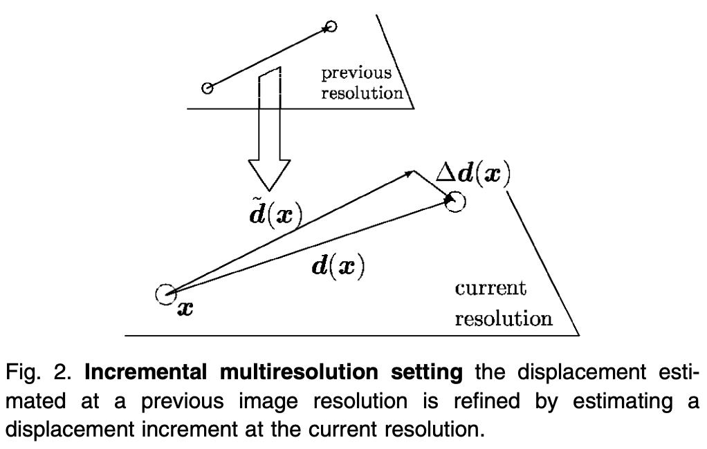
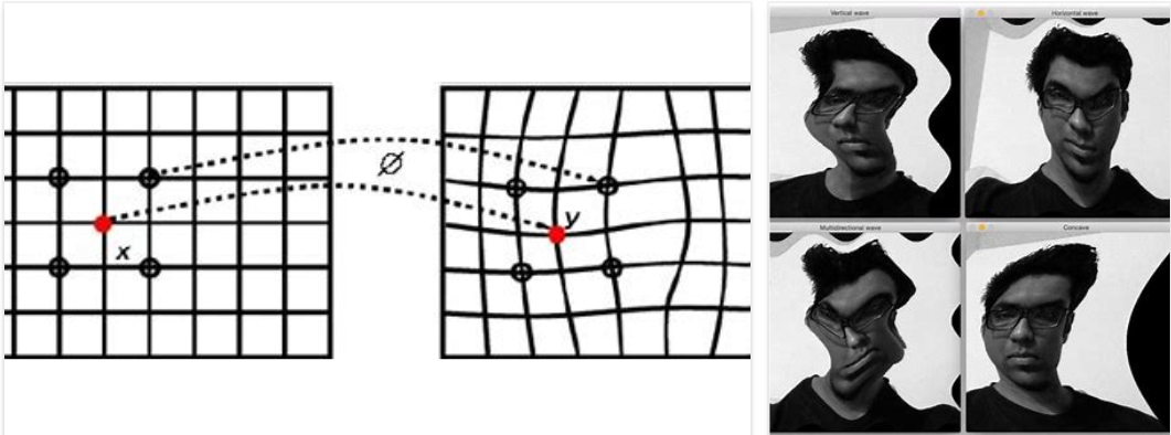
具體執行方式：Given a previous estimate $\tilde{\mathbf{d}}$ of the displacemtn field at a coarser resolution, a first order expansion of the first term in $\eqref{OpticFlowD}$ is performed around $(\mathbf{x}+ \tilde{\mathbf{d}}(\mathbf{x}), t+\Delta t)$，見下圖，會得到以下的 cost function

\[\begin{equation} \int_{\Omega} f_{1}\left[\nabla I(x+\tilde{d}(x), t+\Delta t) \cdot \Delta d(x)+I(x+\tilde{d}(x), \\ t+\Delta t)-I(x, t)\right]+\alpha f_{2}\left[|\nabla(\tilde{d}+\Delta d)(x)|\right] \label{Cost2} \end{equation}\]

to be minimized with respect to the displacement increment $\Delta d=d-\tilde{d}$ (Fig. 2). BTW, 此處的 $\mathbf{d}$ 取代 $\boldsymbol{v}$ 的作用。

Fig. 1 -

$\eqref{Cost2}$ 式基本假設 (i) brightness constancy; (ii) first-order smoothness. 我們接下來修正這兩個假設。

Brightness Constancy 修正 $\to$ Compressible Fluid Continuity Equation

Constant brightness 適用於剛性物體的運動亮度不變。但有例外 (i) 大小會改變的 motion, e.g. 有 depth 方向的移動；(ii) deformable motion, e.g. 氣體，心臟跳動。

修正的方法基於 continuity equation. 先看 fluid continuity equation (conservation of mass)

\[\begin{equation} \frac{\partial \rho}{\partial t}+\nabla \cdot(\rho \mathbf{V})=0 \label{FluidCont} \end{equation}\]

where

• $\rho$ is the fluid density
• $\mathbf{V}$ is the 3D velocity field

我們可以直接利用 $\eqref{FluidCont}$ 類比成 2D 的 image brightness $I$ and velocity $\boldsymbol{v}$ Satisfy:

\[\begin{equation} \frac{\partial I}{\partial t}+\nabla \cdot(I \boldsymbol{v})=0 \label{OpticCont} \end{equation}\]

$\nabla \cdot(I \boldsymbol{v}) = \nabla I \cdot \boldsymbol{v} + I (\nabla \cdot \boldsymbol{v})$. 對於 incompressible flow, i.e $\nabla \cdot \boldsymbol{v}=0$, $\eqref{OpticCont}$ 化簡為一般 optical flow equation $\eqref{OpticFlow}$. 相反對於 compressible flow, $\eqref{OpticCont}$ 比 optical flow equation $\eqref{OpticFlow}$ 多了一項 $I (\nabla\cdot \boldsymbol{v})$. 也就是換成全微分是要加上這多出的一項。

\[\begin{equation} \frac{d I}{d t}+ I \nabla \cdot \boldsymbol{v}=0 \label{OpticCont2} \end{equation}\]

$\eqref{Cost2}$ 也可以對應修正，基本要乘上一個 $\exp (\nabla\cdot \tilde d) $ term, 參考 [@corpettiDenseEstimation2002]. 因為修正主要是對 deformable 移動，i.e. $\nabla \cdot \boldsymbol{v}\ne 0$，此處不再討論細節。

First Order Smoothness 修正 $\to$ Second Order Smoothness

上式 $f_2$ 是 1st order smoothness.

\[\begin{equation} \int_{\Omega}|\nabla u|^{2}+|\nabla v|^{2} \end{equation}\]

the same as those associated with order div-curl regularizer [41]

\[\begin{equation} \int_{\Omega} (\nabla \cdot d)^2 +(\nabla \times d)^2 \end{equation}\]

where $\nabla \cdot \boldsymbol{d}=\frac{\partial u}{\partial x}+\frac{\partial v}{\partial y}$ and $\nabla \times \mathbf{d} =\frac{\partial v}{\partial x}-\frac{\partial u}{\partial y}$

修正為 2nd order smoothness 為 gradient of div-curl regularizer.

\[\begin{equation} \int_{\Omega} |\nabla (\nabla \cdot d)|^2 + |\nabla (\nabla \times d)|^2 \end{equation}\]

Again, 本文主要是討論 AI optical flow, 細節可以參考 [@corpettiDenseEstimation2002].

Optical Flow 變分 Variational Model

參考 [@broxHighAccuracy2004]。

Optical flow variation form 看起來和積分形式一樣。差異是在積分内的函數。因爲是要找積分内函數的最小值，所以稱爲 variational from. 其實積分形式也可以稱爲 variational method.

Variational approach 是從基本上就否定 small displacement and linearization. 而是用 large displacement and warping 取代。

Variational model 爲什麽重要? (1) 因爲這是 CV 算法 SOTA 的結果；(2) 這個方法直接 lead to深度學習的做法。

Variational Metghod Assumption

• Grey value (i.e. lumicent) constancy assumption: 就是 $\eqref{OpticFlowD}$, 注意此處沒有假設 small displacement.

• Gradient costancy assumption: \(\nabla I(x, y, t)=\nabla I(x+u, y+v, t+1)\) Here $\nabla=\left(\partial_{x}, \partial_{y}\right)^{\top}$ denotes the spatial gradient.

• Smoothness assumption

• Multiscale approach: 因爲是 large displacement assumption, cost function 可能會有 local minimum. 如果用 small displacement iteration 有可能會陷入 local minimum. 要找到 global minimu, 一個方法使用 multiscale (resolution) approach. 一開始用 coarse (i.e. lower resolution, larger receptive field), 再持續用 higher resolution to refine the flow. 後面可以看到這對深度學習是很好的機會。因爲深度學習的 encoder/decoder structure 基本就是 multiscale (resolution).

  接下來可以定義 cost function or energy function:

\[\begin{equation} E(u, v)=E_{\text {Data }}+\alpha E_{Smooth} \end{equation}\]

and

\[\begin{equation} E_{\text {Data }}(u, v)=\int_{\Omega} \Psi\left(|I(\mathbf{x}+\mathbf{w})-I(\mathbf{x})|^{2}+\gamma|\nabla I(\mathbf{x}+\mathbf{w})-\nabla I(\mathbf{x})|^{2}\right) \mathbf{d} \mathbf{x} \end{equation}\]

The function $\Psi$ can also be applied separately to each of these two terms. We use the function $\Psi\left(s^{2}\right)=\sqrt{s^{2}+\epsilon^{2}}$ which results in (modified) $L^{1}$ minimisation. With $\gamma$ being a weight between both assumptions. Since with quadratic penalisers, outliers get too much influence on the estimation, an increasing concave function $\Psi\left(s^{2}\right)$ is applied, leading to a robust energy $[7,16]$ : \(\begin{equation} E_{S m o o t h}(u, v)=\int_{\Omega} \Psi\left(\left|\nabla_{3} u\right|^{2}+\left|\nabla_{3} v\right|^{2}\right) \mathbf{d} \mathbf{x} \end{equation}\)

Finally, a smoothness term has to describe the model assumption of a piecewise smooth flow field. This is achieved by penalising the total variation of the flow field $[20,8]$, which can be expressed as with the same function for $\Psi$ as above. The spatio-temporal gradient $\nabla_{3}:=\left(\partial_{x}, \partial_{y}, \partial_{t}\right)^{\top}$ indicates that a spatio-temporal smoothness assumption is involved. For applications with only two images available it is replaced by the spatial gradient. The total energy is the weighted sum between the data term and the smoothness term

爲什麽不用以下 cost function? 因爲不夠 robust against outlier. \(\begin{equation} E_{\text {Data }}(u, v)=\int_{\Omega}\left(|I(\mathbf{x}+\mathbf{w})-I(\mathbf{x})|^{2}+\gamma|\nabla I(\mathbf{x}+\mathbf{w})-\nabla I(\mathbf{x})|^{2}\right) \mathbf{d} \mathbf{x} \end{equation}\)

重點來了：以上的 Euler-Lagrange optimization 可以證明和 warping 等價！[@broxHighAccuracy2004]

Neural Network Optical Flow

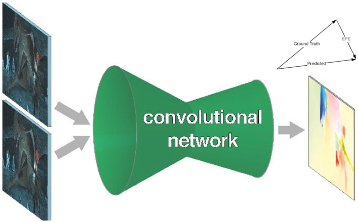
回到 neural network optical flow， 算法的基礎是 end-to-end training of $\eqref{OpticFlowD}$:

• Input 是兩張相鄰 $\Delta t$ 的 frames: $I( \mathbf{x}+ \mathbf{d(x)}, t+\Delta t)$ 和 $I(\mathbf{x}, t)$.
• Output 是 $\mathbf{d(x)}$ 對每個 pixel $\mathbf{x}$.
• 我們使用一個 neural network to model 這個複雜的 input and output function.
• Training 的 cost/loss function 是每個像素的预测的光流（2维向量）和 ground truth 之间的欧式距离，这种误差为 EPE (End-Point-Error)，如下圖右上。

Fig.2 - Optical Flow Neural Network.

Optical Flow Neural Network Model Overview

從2015 年的劃時代意義的 FlowNet (Freiburg University, Germany) 到現在 Sintel 榜單第一 GMA [1]（更新日期：2021.11.29），已有數十篇基於深度學習的光流估計的論文。

FlowNet (and FlowNet2) 是第一個嘗試利用CNN去直接預測光流的工作，它將光流預測問題建模為一個有監督的深度學習問題。 再來的 SPyNet 引入 spatial pyramid of image for coarse-to-fine flow refinement。接下來 PWC-Net (Nvidia) 是經典中的經典，很多光流算法是基於 PWC-Net 的框架來是實現的；而 2020 的 RAFT (Princeton) 則是另一個有劃時代意義的光流算法，也已經有若干篇論文基於它的結構來拓展。

Innovation and Key Feature Summary

Optical Flow Neural Network Model 隨著時間逐步改善。這裏列出各種 Optical Flow Neural Network Model 的 innovations 和 benefits，方便大家看出源流。

Model	Year	Institute	Innovations	Benefit
FlowNet	ICCV2015	xxx, Germany	引入 CNN U-Net 結構 for optical flow	fast computation of CNN compared with CV method
FlowNet2	CVPR2017		(i) Cascaded FlowNet (ii) 引入 warping to refine the flow	good accuracy, but trade-off of model size and computation cost
SPyNet	CVPR2017	Max Planck Institute	Spatial Pyramid of image (+warping) for coarse-to-fine flow refinement, and reduce parameter	save parameters and computation cost.
PWCNet	CVPR2018	Nvidia	(i) Spatial pyramid (+warping) 推廣到 feature space (ii) 引入 cost volume loss 而非只是 feature loss	save parameters and computation cost; higher accuracy compared with SPyNet.
RAFT	ECCV2020	Princeton	(i) RNN for recurrent flow refinement	Small object

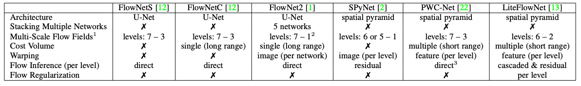
更詳細的 feature 比較表如下。

	FlowNetS	FlowNetC	FlowNet2	SPyNet	PWCNet	LiteFlowNet	RAFT
Architecture	U-Net	U-Net	U-Net	spatial pyramid	spatial pyramid	spatial pyramid	RNN
Stacking Multiple Networks	x	x	5 networks	x	x	x	Game Super Resolution
Multi-Scale Flow Fields¹	levels: 7-3	levels: 7-3	levels: 7-1	levels: 6 or 5-1	levels: 7-3	levels: 6-2	?
Cost Volume	x	single (long range)	single (long range)	x	multiple (short range)	multiple (short range)	?
Warping	x	x	image (per network)	image (per level)	feature (per level)	feature (per level)	feature?
Flow Inference (per level)	direct	direct	direct	residual	direct	cascaded & residual	direct?
Flow Regularization	x	x	x	x	x	per level	x
Parameter			162M	9.7M	8.8M	5.4M

Network Structure

以下介紹這幾種算法的模型結構。

先來定義一下後面會用到的符號。光流估計是計算圖像之間的運動，對於圖像 $img_1$ 和 $img_2$ 之間的光流 $w \in R^{H\times W\times 2}$ ，它的每個位置上的二維向量表示了 $img_1$ 上的某一個點 $p_{x1}$ 到 $img_2$ 上相同一點 $p_{x2}$ 之間的偏移，下標 $x$ 表示圖像上的坐標。通俗來講，光流描述了圖像之間，每個像素點的運動軌跡。下文的敘述中，有些也會用 $w$ 代表光流某個位置上的值，即偏移的二維向量。

FlowNet(1.0) (CNN-base, 2015)

FlowNet(1.0) 的結構非常單純，就是 brute force 的 CNN end-to-end training.

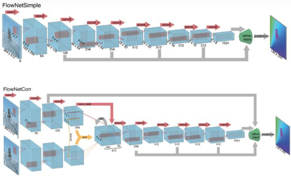
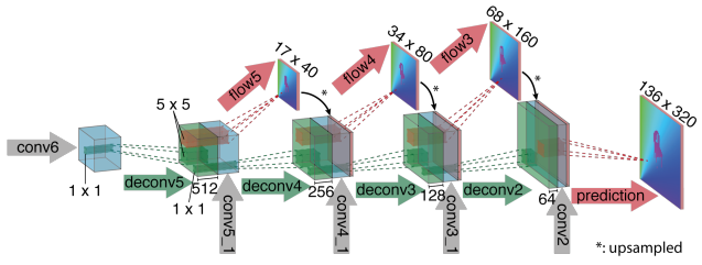
FlowNet(1.0) 的 CNN 結構是 encoder (Fig. 3) + decoder (Fig. 4). Fig. 3 包含兩種不同的 encoders. Encoder 都是用 Fig. 4.

Q: Why the aspect ratio is changed for encoder and decoder?

FlowNetS (Simple) and FlowNetC (Corr)

Building block 其實就是 CNN encoder+decoder: encoder 共有 9 級，分辨率逐級減半，不過有些級分辨率不變。decoder 有 4 級，每級解析度倍增。這個架構類似 U-Net 架構。可以參考前文 “Computer Vision - UNet from Autoencoder and FCN“. FCN and U-Net 原來用於 image segmentation, 之後廣泛用於 pixel image processing 例如 super resolution, noise reduction, etc.

FlowNetS 和 FlowNetC 主要的差別是在 input stage.

• FlowNetSimple 直接將兩張圖像按通道維重疊後輸入。
• FlowNetCorr 為了提升網絡的匹配性能，人為模仿標準的匹配過程，設計出「互相關層」，即先提取特徵，再計算特徵的相關性。相關性的計算實際上可以看做是兩張圖像的特徵在空間維做卷積運算。
• FlowNetC 的計算量顯然大於 FlowNetS. 但是效果也比較好。在 FlowNet2.0 只用於 input stage for large displacement estimation. 其餘兩個 stages 只需要用比較簡單的 FlowNetS.

Fig. 3 - FlowNet Encoder: 上圖 FlowNetSimple; 下圖 FlowNetCorr.

Fig. 4 - FlowNet Refinement/Decoder Network.

FlowNet2 (Cascade FlowNet + Warping, 2016)

參考 [@sigaiFlowNetFlowNet22019]

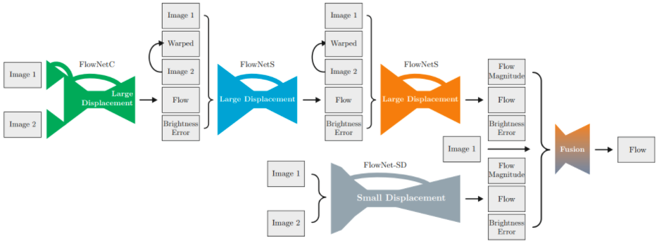
• 先鳥瞰 FlowNet2 的結構如下圖，包含四個 CNN-based optical flow estimators: 其中三個 large displacement (1xFlowNetC, 2xFlowNetS building block of FlowNet1) 組成 cascaded networks.

• FlowNet2 的另一個關鍵是利用 warping 讓 image2 逐步接近 image2 (iterative estimation) 概念如同 $\eqref{Cost2}$.

• 最後一個 small displacement (1xFlowNet-SD). FlowNet2 的改進就是一再修正 $\Delta d$, 三個大的修正再和小修正 fuse 一起。
• FlowNet 另外還會估計 brightness error 修正 constant brightness 假設。

細節：

• FlowNetC: Image1(t) - Image2(t+dt) $\to$ Large displacement estimation
• FlowNetS1: Image1(t) - Image2(t+dt - backwarp1) $\to$ Large displacement estimation1
• FlowNetS2: Image1(t) - Image2(t+dt - backwarp2) $\to$ Large displacement estimation2

Fig.5 - Schematic view of FlowNet2.0. To compute large displacement optical flow we combine multiple FlowNets. 大括號代表 inputs concatenation. Brightness Error is the difference between the 1st image and the 2nd image warped with the previously estimated flow. To optimally deal with small displacements, we introduce smaller strides in the beginning and convolutions between upconvolutions into the FlowNetS architecture. Finally we apply a small fusion network to provide the final estimate.

FlowNet1 主要的問題：準確度不夠高。

FlowNet2 主要的問題：準確度不錯。但因爲利用四個 CNN 做 flow iterative refinement, 需要大量的 weight parameters (160M), 在 edge device 造成 memory access bottleneck.

SPyNet (Spatial Pyramid + Warping, 2016)

SpyNet 主要想解決兩個問題 [@ranjanOpticalFlow2016]：

• FlowNet2 利用四個 CNN cascading 做 optical flow iterative refinement. 需要大量參數 (160M).
• 作者觀察採用2幀圖片堆疊的方法，當兩幀圖片之間的運動距離大於1 (或幾個) pixel的時候，CNN 很難學習到有意義的 filter.

Solution:

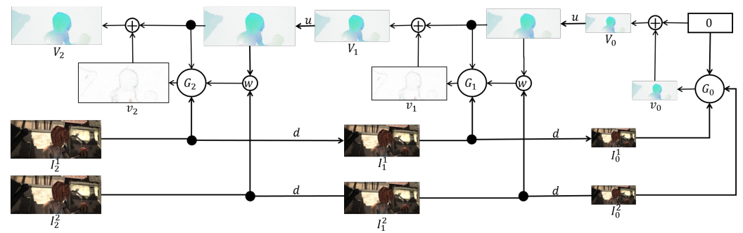
• Spatial pyramid of image (not feature map) to perform coarase-to-fine flow refinement, 如下圖。

• 原始的 Image1 和 Image2 是 $I^1_2$ and $I^2_2$, 上標是 image number, 下標是 image size: 2 (大) $\to$ 1 (中) $\to$ 0 (小)，$d(\cdot)$ 代表 down-sampling/decimating by 2 (長和寬)。相反 $u(\cdot)$ 則是 up-sampling by 2.

• ${G_0, G_1, …, G_k}$​ 是一系列從小變大的 optical flow CNN models. $G_k$​ 有三個 inputs：包含對應 size 的 image1, $I_k^1$​. 以及 warped image2, $w(I^2_k, \text{coarse displacement})$​. $w(\cdot)$​ 是 warping operation¹.

  還有 up-sampling 的 coarse flow, $u(V_{k-1})$​, why? $G_k$​ 的 output 是兩個 images 的 residual flow, $v_k$​.

\[\begin{equation} v_{k}=G_{k}\left(I_{k}^{1}, w\left(I_{k}^{2}, u\left(V_{k-1}\right)\right), u\left(V_{k-1}\right)\right) \label{SpyFlow1} \end{equation}\]

• Refined flow, $V_k$, 就是把 up-sampling corase flow, $V_{k-1}$, 再加上 residual flow 如下。

\[\begin{equation} V_{k}=u\left(V_{k-1}\right)+v_{k} \label{SpyFlow2} \end{equation}\]

• 整個過程是從 $G_0$ 開始：先針對最小 size images $I^1_0$ 和 $I^2_0$ (coarse and no warping) 得到 $v_0 = V_0$ coarse flow. 再 up-sampling $V_0$ 有三個目的 (1) warp $I^2_1$; (2) 輸入 $G_1$ (why?); (3) up-sampled coarse flow 再加上 residual flow, $v_1$, 得到 refined flow $V_1$. 重複這個過程得到 $V_2$, 就是 final flow.

這是一石兩鳥的方法。先從 coarse frames 抓出 coarse flow (large displacement), 再放大 image and resolution 繼續 refine coarse flow to finer flow. 再者 $G_0$ 的 network size and parameter < $G_1$ < $G_2$. 因此全部網路的 parameter size 遠小於 FlowNet2.

Spatial pyramid + warping 的 coarse-to-fine flow 是一個不錯的 idea, 之後用於 PWCNet 和 LiteFlowNet, 而且不限於 image warping, 連 feature map 也一起 warping. 缺點是對於 small object 的 displacement 有可能會 missed.

Fig. 6 - Spatial pyramid: Image (not feature) pyramid from left to right. Flow refinement from right (coarse) to left (fine).

下一個經典網絡是 PWCNet, 基於 FlowNet 和 SpyNet

利用 image+feature warping in each pyramid level 可以節省大量 weight parameters (1.2M or 8.8M?) 從而加速 flow 計算。不過 PWCNet 的精確度大約於 FlowNet, 比 FlowNet2 差。

PWC-Net

[@openmmlabOpticalFlow2021]

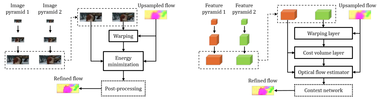
PWC-Net 的設計遵循了三個簡單而成熟的原則： P-金字塔處理，Warping 操作，和 C-代價計算 (cost volume)。在傳統算法中，如圖１左部分所示，通過代價計算得到圖像之間的相似度，構建圖像金字塔，以處理對不同尺度的光流，再利用 warp 操作按 coarse-to-fine 的順序，將上一層估計出的光流應用到當前層，以達到逐級優化的目的。PWC-Net 基於傳統算法的框架設計了如圖１右部分所示的模型結構：

Fig. 7 - Traditional coarese-to-fine approach vs. PWC-Net. 左: Image pyramid and refinement at one pyramid level by the energy minimization approach. 右: Feature pyramid (從下到上，底層為輸入影像) and flow refinement (從上到下) at one pyramid level by PWC-Net. PWC-Net warps features of the second image using the upsampled flow, computes a cost volume, and process the cost volume using CNNs. Both post-processing and context network are optional in each system. The arrows indicate the direction of flow estimation and pyramids are constructed in the opposite direction.

PWC 是以下的縮寫：

1. Pyramid of feature (not only image as Spynet)

   用共享參數的 CNN 模型分別提取兩張圖片 $I_1$ 和 $I_2$ 的特徵金字塔，$c^l_t$ 代表 $I_t$ 在第 $l$ 層的特徵，隨著金字塔層數的增加，特徵尺寸逐步減小，每層尺寸都是上級尺寸的二分之一，約定第 0 層 (底層) 的特徵為輸入圖像，i.e. $c^0_t = I_t$

2. Warping layer (單向把 $c^l_2$ warp 到 $c_1^l$)

   在第 $l$ 级，利用 up-sampling 的 $l+1$ 级光流對 $c^l_2$ 進行 warping 操作，得到 $c^l_w$ 特徵，使當前層從一個比較好的“起點”開始，也是對上層光流進行 refine。這和 SPyNet 相同，只是從 image (in SPyNet) 擴展到 feature map (in PWCNet).

   \[\mathbf{c}_{w}^{l}(\mathbf{x})=\mathbf{c}_{2}^{l}\left(\mathbf{x}+up\left(\mathbf{v}^{l+1}\right)(\mathbf{x})\right) \label{PWCFlow1}\]

   where $\mathbf{x}$ 是 pixel 坐標，$\mathbf{v}^{l+1}$ 是 $l+1$ 光流，and $up(\mathbf{v}^{l+1})(\mathbf{x})$ 是對應位置 up-sampling 的 $l+1$ 層光流。 $\mathbf{c}{w}^{l}(\mathbf{x})$ 就是 $\mathbf{c}{2}^{l}$ backwarp(?) $(\mathbf{x}+\mathbf{w})$ 之後的結果，如下圖。

   

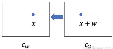
   Fig. 8 - Warping Function.

   如果 $up(\mathbf{v}^{l+1})(\mathbf{x})$ 是準確而且沒有遮擋 (occlusion), $\mathbf{c}{w}^{l}$ 和 $\mathbf{c}{1}^{l}$ 應該是相同的。但這兩者都不成立，因此這裏 coarse-to-fine warping 的目的就是把上層較爲粗糙的 flow，經過一再的 refinement 得到最後的 flow。最上層的 flow 設爲 0, 然後往下 refine the upsampled flow $up(\mathbf{v}^{l+1})(\mathbf{x})$. 我們用 bilinear interpolation to implement the warping operation and compute the gradients to the input CNN features and flow for backpropagation. $\eqref{PWCFlow1}$ 其實和 SPyNet 的 $\eqref{SpyFlow1}$ 的 warping term 基本是相同的意義。

3. Cost volume layer

   計算每層特徵之間的匹配代價，或稱為相關性（correlation）.

   \[\mathbf{c v}^{l}\left(\mathbf{x}_{1}, \mathbf{x}_{2}\right)=\frac{1}{N}\left(\mathbf{c}_{1}^{l}\left(\mathbf{x}_{1}\right)\right)^{\top} \mathbf{c}_{w}^{l}\left(\mathbf{x}_{2}\right) \label{CostV}\]

   where T is the transpose operator and $N$ is the length of the column vector $\mathbf{c}{1}^{l}\left(\mathbf{x}{1}\right)$. 爲了要節省計算 for an $L$-level pyramid setting, we only need to compute a partial cost volume with a limited range of $d$ pixels, i.e., $\left

   \mathbf{x}{1}-\mathbf{x}{2}\right

   _{\infty} \leq d$.

   A one-pixel motion at the top level corresponds to $2^{L-1}$ pixels at the full resolution images. Thus we can set $d$ to be small. The dimension of the $3 \mathrm{D}$ cost volume is $d^{2} \times H^{l} \times W^{l}$, where $H^{l}$ and $W^{l}$ denote the height and width of the $l$ th pyramid level, respectively.

所以 neural network 到底在哪裏? 除了在 (1) feature pyramid, 另外還在 (2) optical flow estimator, a multi-layer CNN.

• Optical flow estimator

  光流估計的子網絡將特徵的 cost volume $\eqref{CostV}$, features of first image $c_1^l$, and upsampled optical flow $up_2 (w_{l+1})$ 拼接在一起作為輸入，輸出當前層的光流 $V^l$ at the $l$-th level，每級網絡的之間不共享參數。這部分概念和 $\eqref{SpyFlow1}$ 以及 $\eqref{SpyFlow2}$ 結合一起類似。參考 Fig. 5.

• Context network

  PWC-Net 對每級特徵都進行類似的 warping-correlation-flow estimation 的操作，直到 $l_2$ 級。在傳統的光流估計算法中，會使用紋理信息對估計出的光流進行後處理。PWC-Net 最後設計了一個 由膨脹卷積組成的 context network（可以擴大感受野）， 將 $l_2$ 級輸出光流前的特徵餵進去，得到 refined flow。將 refined flow 從 $l_2$ 級直接上採樣到原始尺寸，為啥是 $l_2$ 級，這是從 FlowNet 就開始的「慣例」，按 FlowNet 論文作者的解釋，他們比較了將 $l_2$ 級的光流上採樣到原圖尺寸和接著 warping-correlation-flow estimation，發現結果上並沒有明顯的差距，但計算量降低了許多。

  借鑑傳統光流算法的框架設計出來的 PWC-Net 模型是非常簡潔且高效的，因此後續的算法大多是在此基礎上實現的，直到2020 年的 RAFT，跳出了這個框架，也大幅度刷新了 SOTA 的記錄。

LiteFlowNet (UK, 2018)

[@huiLiteFlowNetLightweight2018]

Fig. 9 -

RAFT: All pairs correlation + recurrent refinement (CNN+RNN)

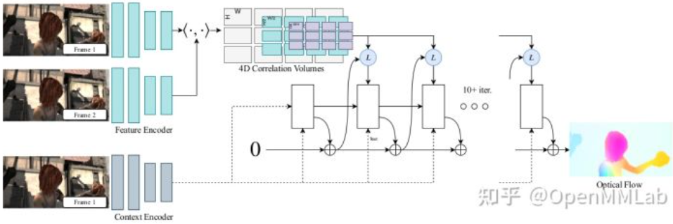
RAFT 是 ECCV2020 的 best paper，將一種全新的模型結構引入到光流領域。它的模型由三個部分組成：(Fig. 7)

1. 特徵提取 (feature extraction) 這部分也是利用共享參數的 CNN 提取兩張圖像的特徵，不同是的輸出的不是圖像金字塔，而是長寬為原圖 1/8 的特徵。另外用一個結構相同的網絡，再提取一份 $I_1$ 的特徵，作為 context 特徵。

2. 相關性計算 與之前計算局部的相關性 (e.g. PWCNet cost volume?) 不同，RAFT 計算兩個特徵所有像素之間的相關性 all-pairs correlation。如果圖像的特徵為 $c_1 \in R^{H\times W \times C}$ 和 $c_2 \in R^{H\times W \times C}$ ，則相關性 correlation volume 為 [公式] ，是逐像素特徵表達之間的內積。再對 [公式] 的後兩維 avg pooling 下採樣多次，得到 correlation pyramid [公式] , [公式]

3. 循環迭代更新 論文中解釋這部分的設計是在模仿優化過程，逐次優化使得 [公式] 。每次輸入上次估計的光流 [公式] , correlation 和 hidden state，輸出 [公式] ，則當前的估計的光流為 [公式] 。默認初始化 [公式] 為0，hidden state 是 context feature，循環的單元選擇的是 GRU cell，訓練時的迭代次數為12次。由此估計出的光流的大小是 [公式] ，其中 [公式] 和 [公式] 是原圖的尺寸，需要進一步對輸出的光流上採樣以得到原始尺寸大小的光流。RAFT 使用低解析度下鄰域像素光流的線性組合來恢復尺寸，具體做法是，將當前 GRU cell 輸出的 hidden state 輸入到一個小網絡中，預測一個 [公式] mask，對 [公式] flow 提取 [公式] 的局部鄰域塊，如下圖所示，用 mask 對 flow 的鄰域加權求和，每個鄰域的 mask 有64個，所以再 reshape 就可以得到原圖大小的光流。

Fig. 10 -

RAFT 幾個創新點：

1. 先前的框架普遍采用從粗到細的設計 (e.g. Pyramid in PWCnet)，也就是先用低分辨率估算流量，再用高分辨率采樣和調整。

相比之下，RAFT以高分辨率維護和更新單個固定的光流場。

這種做法帶來了如下幾個突破：低分辨率導致的預測錯誤率降低，錯過小而快速移動目標的概率降低，以及超過1M參數的訓練通常需要的叠代次數降低。

1. 先前的框架包括某種形式上的叠代細化，但不限制叠代之間的權重，這就導致了叠代次數的限制。

例如，IRR 使用的 FlowNetS 或 PWC-Net作為循環單元，前者受網絡大小（參數量38M）限制，只能應用5次叠代，後者受金字塔等級數限制。

相比之下，RAFT的更新運算是周期性、輕量級的：這個框架的更新運算器只有2.7M個參數，可以叠代100多次。

1. 先前框架中的微調模塊，通常只采用普通卷積或相關聯層。

相比之下，更新運算符是新設計，由卷積GRU組成，該卷積GRU在4D多尺度相關聯向量上的表現更加優異。

FlowNet / SPyNet / PWCNet / RAFT Key Features Comparison

Fig. 4 - Key Features of Different NN Optical Flow Method

• Warping 是 image level or feature level is another key!

	FlowNetS	FlowNetC	FlowNet2	SPyNet	PWCNet	LiteFlowNet	RAFT
Architecture	U-Net	U-Net	U-Net	spatial pyramid	spatial pyramid	spatial pyramid	RNN
Stacking Multiple Networks	x	x	5 networks	x	x	x	x
Multi-Scale Flow Fields¹	levels: 7-3	levels: 7-3	levels: 7-1	levels: 6 or 5-1	levels: 7-3	levels: 6-2	?
Cost Volume	x	single (long range)	single (long range)	x	multiple (short range)	multiple (short range)	?
Warping	x	x	image (per network)	image (per level)	feature (per level)	feature (per level)	feature?
Flow Inference (per level)	direct	direct	direct	residual	direct	cascaded & residual	direct?
Flow Regularization	x	x	x	x	x	per level	x
Parameter			162M	9.7M	8.8M	5.4M

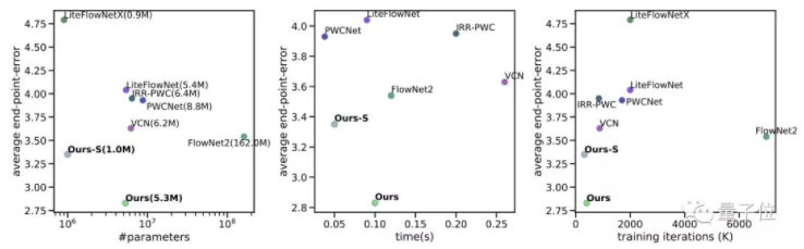
FlowNet / PWCNet / RAFT Performance Comparison

NN optical flow FlowNet 算法基本已經和 SOTA CV optical flow 算法打平。接下來的 PWCNet 和 RAFT 的 performance 愈來愈好，已經是一騎絕塵。In terms of accuracy: RAFT > FlowNet2 > PWCNet ~ FlowNet. Average EPE (End-Point-Error) vs. parameter # / time / training iterations 如下。

Fig. 11 -

CORRESPONDENCES BETWEEN OPTICAL FLOW CNNS AND VARIATIONAL METHODS

We first provide a brief review for estimating optical flow using variational methods. In the next two sub-sections, we will bridge the correspondences between optical flow CNNs and classical variational methods.

The flow field can be estimated by minimizing an energy functional E of the general form

Search and Match problem

to avoid overfitting.

Three method to conquer the big displacement problem:

1. Iterative method but same resolution: RAFT (local minimum?)
2. Pyramid method with multi-resolutoin: low resolution to get the flow; then high resolution to refine the flow to flux
3. 1+2 => FlowNet2? but with very limited iteration (2 - 3 times)

Appendix

Warping Operation and MEMC

1. Warping operation $w(\cdot)$ 不是一種 function.

它是改變定義域 $T:\mathbf{x} \to \mathbf{x’}$，而不是像函數 define 值域 $f:\mathbf{x} \to y$.

傳統的 image warping 是 stationary image warping，1-to-1 mapping from $x \to x’$, 沒有 motion 造成的位移 (offset) 和遮蔽 (occlusion)，只是坐標的變換或扭曲。常見的綫性坐標轉換是 affine transform: $\mathbf{x’} = \mathbf{A} \mathbf{x’} + \mathbf{B}$. 不過説到 warping 一般是指非綫性坐標轉換。

Fig. 1 -

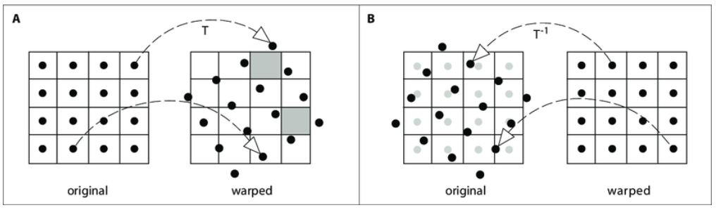
2. Warping operation 分爲兩類：foward warping $T$ (下圖左) and backward warping $T^{-1}$ (下圖右)。

假設簡單的 1-to-1 mapping of $T$。這種簡單的 mapping, 原則上 $T T^{-1} = I$，也就是 $T$ and $T^{-1}$ are reversable，可以視爲坐標變換。但是因爲作用在不同的 images grid 上：$T$ is on orignal image; $T^{-1}$ is on warped image，兩者還是有一些不同，不是完全 reversable, 如下圖 A and B.

Forward warping, $T$, is based on the orignal image, 如下圖 A。在產生 warped image 會有 (1) pixel lands between two pixels; (2) holes problem.

Backward warping, $T^{-1}$, is based on the warped image, 如下圖 B。只要在 original image 做 interpolation 即可。所以一般都是用 backward warping or inverse warping.

Fig.12 - Forward and backward image warping. (A) Foward warping, holes can occur in the warped image, marked in gray. (B) Backward warping eliminates this problem since intensities at locations that do not coincide with pixel coordinates can be obtained from the original image using an interpolation scheme.

3. Motion Warping With Occulsion (Not 1-to-1 Mapping)

本文主要討論 optical flow, 也就是 motion. Motion 對應的 warping 一般會有移動 (offset) 和遮蔽 (occlusion). 這會讓 forward flow 和 backward flow 不會互爲 reverse，因爲 motion 的關係會作用在不同的坐標點。此時用 $T$ 和 $T^{-1}$ 很容易誤導。因此我們會用 $T_{A\to B}$ 和 $T_{B\to A}$ 代表 forward flow 和 backward flow。當然 $T_{A\to B} \ne T_{B \to A}^{-1}$.

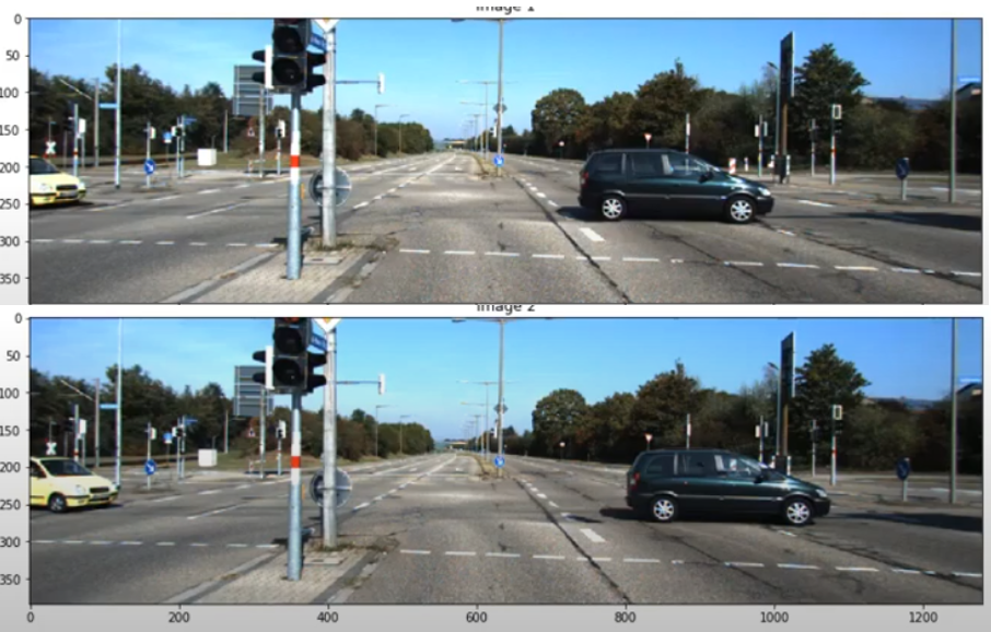
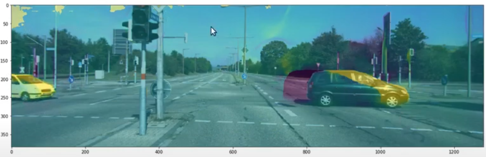
我們看一個簡單的例子。Fig. 12 車從 A (image1) 移動到 B (image2)。從 image1 的角度，除了車子 pixels 有移動以外，其他所有的 pixel 都是靜止。如 Fig. 13 中的 $T_{A\to B}$ 紫色部分，代表向右移動。從 image 2 的角度，也是只有車子 pixel 有移動，但是相反的方向。因此 $T_{B\to A}$ 如 Fig. 13 黃色的部分。非常重要：紫色和黃色的部分方向雖然相反，但是因爲移動的關係，兩者的位置不完全重叠。也就是 $T_{B\to A} \ne T^{-1}_{A\to B}$.

再來看 occlusion 的問題：original image1 A 點車的 flow vector (右向 vector) 和 B 點號誌桿的 flow vector (0 vector) 會在 warped image 的 B 點對應到同一點。如果車在號誌桿前 (as in this case)，車會遮蔽號誌桿，反之號誌桿會遮蔽車。就是forward warping 還需要 depth map 才能從 image1 + forward motion $T_{A\to B}$ 得到 warped image2.

另一個問題是 A 點在車移動之後需要無中生有一些東西填補背景。爲 image inpainting. 一般是用 original image A 點附近的 pixels 填補。

Fig. 12 - Up:Image1 and Down:Image2

Fig. 13 - Motion Vector of A to B (紫色), and B to A (黃色)

同樣我們可以用 Image2 + backward motion $T_{B\to A}$ 得到 image1. 基本和 original image1 + $T_{A\to B}$ 得到 image2 一樣，只是 time reverse. 但我們真正想要探討的是 Image1 + backward motion $T_{B\to A}$ 得到 image2, 稱爲 backward warping or inverse warping.

Original image1 + backward motion 不需要 depth map 就可以得到 image2. 因爲 warped image 的 B 點的 $T_{B\to A}$ 只會指到 original image 的 A 車。不過這時會遇到的問題是 warped image 的 A 點沒有 $T_{B\to A}$ ! 還是需要無中生有填補一些東西作爲背景，(inpainting)，一般是用 warped image 附近的 pixels 填補。

總結 no-motion and motion 以及 forward warping and backward warping 如下表。一般使用 original image1 + backward motion $T_{B\to A}$ , 因爲 spatial interpolation 或是 background inpainting 都比較容易。

Warping	兩張影像無相對運動	兩張影像有相對運動 with (i) motion (ii) occulsion
坐標變換	1-to-1 mapping, reversable, $T$ and $T^{-1}$	Non 1-to-1 mapping due to (i) motion; (ii) occulsion. $T_{A\to B}$ and $T_{B\to A} \ne T_{A\to B}^{-1}$
Warping function	Linear or nonlinear continuous warping $T$	Non-continuous warping $T_{A\to B}$. 只有 motion 部分有 warping, 沒有 motion 部分無 warping
Forward Warping	Image1 + $T \to$ Image2	Image1 + $T_{A\to B} \to$ Image2
Foward Warping Issues	- Pixel lands between two pixels - Holes problem - Need splatting	- Need depth map for occlusion - Need image inpainting background
Backward Warping	Image1 + $T^{-1} \to$ Image2	Image1 + $T_{B\to A} \to$ Image2
Backward Warping Issues	Need spatial interpolation of image1 (easy and well known)	Need image inpainting background, but no need of depth map

注意！backward warping 不是 Image2 + $T_{B\to A} \to$ Image1! 這只是另一種 forward warping but reverse time sequence.

Motion Estimation Motion Compensation (MEMC)

Optical flow 的一個主要應用是 MEMC，就是所謂插幀。基本所有的電視都有這個功能。就是從 $I_{t-1}$ 和 $I_{t+1}$ 内插出 $I_t$​. 這個插幀可以在正中間，例如 30 FPS to 60 FPS; 或是 60 FPS to 120 FPS. 也可以不在正中間，例如 24 FPS to 60 FPS.

MEMC 顧名思義包含 ME (Motion Estimation) 和 MC (Motion Compensation).

ME 基本有三類: (i) conventional ME (此處不論); (ii) optical flow motion estimation (pixl level); (iii) kernel (patch level) (也不論)。

MC 包含: image warping，image inpainting.

因爲深度學習的 optical flow motion estimation 已經包含 image/feature warping, 因此 ME 和 MC 可以合在同一個網路。就是把原來 optical flow network for motion estimation 擴大 to cover 完整的 MEMC network。

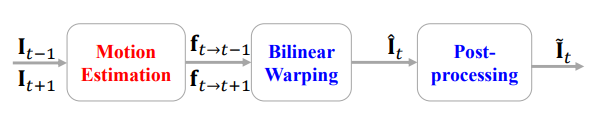
基本可以把 MEMC 分爲三個 steps，如下圖： [@baoMEMCNetMotionEstimation2019]

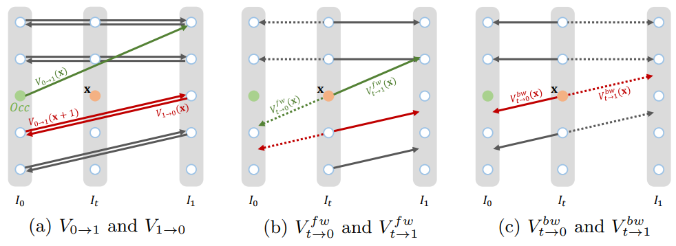
Step 1: 我們可以從 $I_{t-1}$ 和 $I_{t+1}$ 得到 forward optical flow $f_{t-1\to t+1}$, 和 backward optical flow $f_{t+1\to t-1}$.

Step 2: 再來是從 step 1 的 optical flow 内插 $f_{t\to t-1}$ 和 $f_{t\to t+1}$

Step 3: 接下來觀念上可以用 $I_{t-1} + f_{t\to t-1}$ backward warping 得到 $I_t$. 同樣用 $I_{t+1} + f_{t\to t+1}$ backward warping 得到 $I_t$. 當然這兩個結果還是會有差異。因此觀念上可以做 bilaterial warping 得到更好的結果。

接下來會看一些例子。

Ex1: MEMC-Net (2019)，ME is based on FlowNetS

[@baoMEMCNetMotionEstimation2019] 下圖是 MEMC-Net architecture. 最上面的分支就是 Motion Estimation.

ME part

Step 1: Motion estimation 直接用 FlowNetS in Fig. 3. Input: $I_{t-1}, I_{t+1}$, output: $f_{t-1\to t+1}, f_{t+1\to t-1}$.

Step 2: 用 flow projection layer, input: $f_{t-1\to t+1}, f_{t+1\to t-1}$, output $f_{t\to t+1}, f_{t\to t-1}$. 基本假設 linear motion projection.

MC part

Warping : motion warping + kernel warping

Inpainting: 因爲有兩張 frames, 一般會有 1 frame occlusion 可以被另一 frame cover. 所以只要標出 Occulusion mask 配合 warping 即可。最後如 PWCnet 再加上 context network for post processing.

再看一個例子，BMBC:

Ex2: BMBC (Bilateral Motion Estimation with Bilateral Cost Volume, 2020), based on PWCNet

[@parkBMBCBilateral2020] 下圖是 BMBC archtecture. 上三路的 (shared) bilateral motion network 是最重要的 building block to perform Motion Estimation (ME)。之後的 warping layer 和第四路的 context extractor 則是 perform Motion Compensation (MC)。

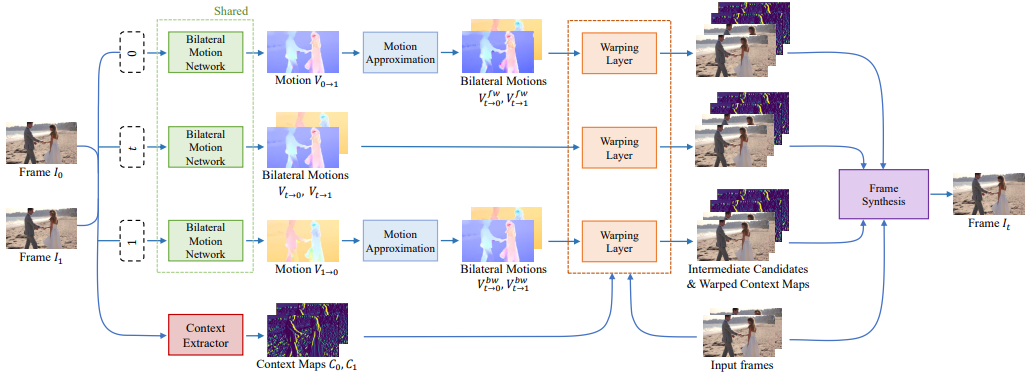
ME part

Combine Step 1 and 2: Bilateral Motion Estimation，如下圖。這裏把 step 1 和 2 結合一起，直接得到 $V_{t\to 0}$ 和 $V_{t\to 1}$，如下圖。

其實是把 PWCnet 加上改良，把原來 Pyramid1 warp to Pyramid0 部分，再加上 Pyramid0 warp to Pyramid1 (改良 bilateral 部分)。比較巧妙的部分是直接把兩個改成 Pyramid1/2 warp to Pyramid t. 並且得到 $V^l_{t\to 0}$ and $V^l_{t\to 1}$。 注意這裏都是用 backward warping!

Fig.15 - Bilateral Optical Flow Motion Estimation： 這裏的架構和 Fig.7 相同，但從單向 Pyramid2 warp to Pyramid1 改成雙向 Pyramid1/Pyramid2 warp to Pyramid t.

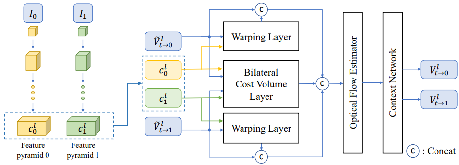
Cost Volume 的做法也是變成雙向。$d$ 是 search window size $D = [-d, d] \times [-d, d]$ 爲了減小 computation complexity. \(B C_{t}^{l}(\mathbf{x}, \mathbf{d})=c_{0}^{l}\left(\mathbf{x}+\widetilde{V}_{\mathrm{t} \rightarrow 0}^{l}(\mathbf{x})-2 t \times \mathbf{d}\right)^{T} c_{1}^{l}\left(\mathbf{x}+\widetilde{V}_{\mathrm{t} \rightarrow 1}^{l}(\mathbf{x})+2(1-t) \times \mathbf{d}\right)\)

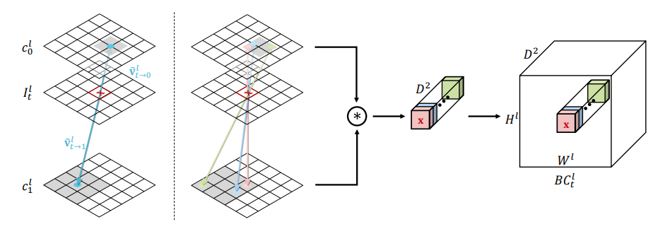
注意 $V_{0\to 1}$ 或是 $V_{1\to 0}$ 只是 $t=0$ 或是 $t=1$ 的特例。就回到 PWC-Net.

那麽上上圖的 branch 1 and 3 的 Motion Approximation 是要做什麽? 主要是針對 occlusion 再產生更多的 $V_{t\to 0}$ 和 $V_{t\to 1}$，如下圖。細節請直接參考 paper.

Fig.13 - Motion approximation： bi-directional motions in (a) are used to approximate forward bilateral motions in (b), and backward bilateral motions in (c).

再來非常複雜的把三路中每一路的 4 張 estimated Image t, 連同 2 張 input image, 一共 4x3+2 = 14 張合成 $I_t$. 應該是不計計算成本。

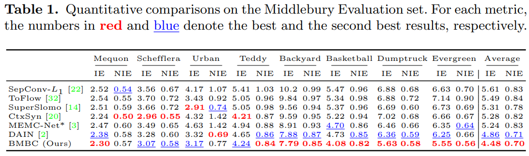
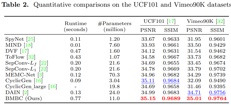
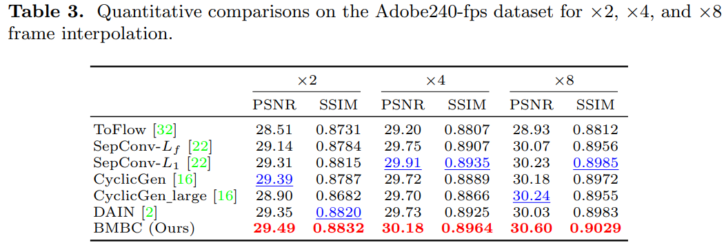
實驗結果

用了 4 組 datasets, Middlebury, Vimeo90K, UCF101, Adobe240-fps. 並且比較 SOTA 結果。

• Adaptive convolution: SepConv, ToFlow, CtxSyn
• Optical Flow NN: ToFlow, SPyNet, MEMC-Net (Bao), DAIN (depth aware, Bao), BMBC

Middlebury

1. 參考 PWCNet 的 warping operation. ↩