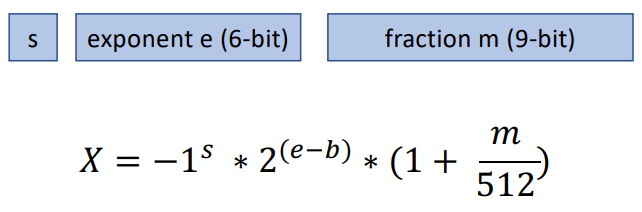
Floating Point representation s: signed bit for mantissa; m: (unsigned) mantissa; e: (unsigned) exponent, b: fixed exponent bias, 因此 e-b 就會是 signed exponent.
-
$f = (-1)^s 2^{e-b} (1+\frac{d_1}{2}+\frac{d_2}{2^2}+\ldots+\frac{d_m}{2^m})\quad$ where $d_i \in {0, 1}$
-
sign-bit 非常簡單直觀,是 mantissa 的正負號,和 exponent 無關。
- 負值只是乘 (-1). 浮點的正負值完全對稱,這和 integer 的 2’s complement 有點不同。
- 所以 floating point 有 +0 和 -0! $[000…0] \to +0\,;\quad [100…0]\to -0.$
-
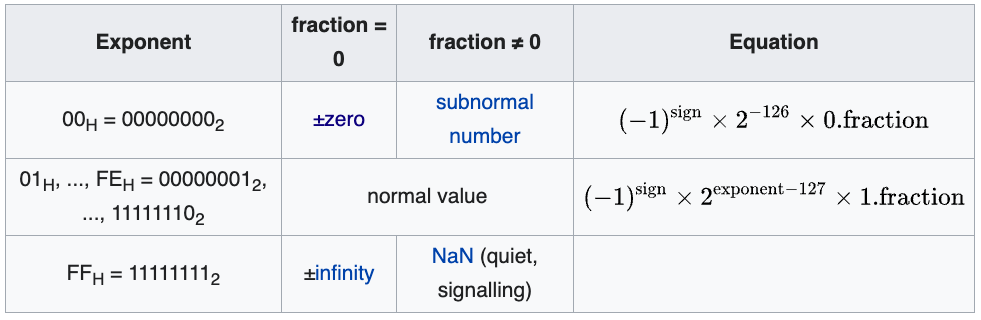
Unsiged mantissa 的 range 是 $[1, 2-\frac{1}{2^m}] \sim [1,2]$: leading 1 是 default, 沒有 encode 在 mantissa!
- 但是在 subnormal (i.e. exponent = 0) 情況下: leading 1 變成 0. 但是要調整 exponnet (+1) 吸收這部分。
-
Biased exponent (最容易搞錯的地方):
- exponent (e) 的範圍:$ [0, 2^{exp\, bit}-1]$
- bias (b) 固定是上述 range 的 mid-point:$2^{exp\,bit}/2-1 = 2^{exp\,bit-1}-1$
- 所以 (e-b) 的範圍: $[-2^{exp\, bit-1}+1,..,+2^{exp \,bit-1}]$
- 不過 exponent 的最小和最大值都被保為不同的用途,所以 (e-b) 實際的範圍 $[-2^{exp\, bit-1}+2,..,+2^{exp \,bit-1}-1]$
- 最小值 (exponent = 0, i.e. all exponet bit = 0) 保留為 subnormal value, mantissa leading 1 變成 0.
- +/-0 是 subnormal (all exponent bit = 0) 的 speical case. 所有 mantissa bit = 0. Sign-bit 0 就是 +0, sign-bit 1 就是 -0.
- 最大值保留為 +/-inf. Sign-bit 0 就是 +inf, sign-bit 1 就是 -inf.
-
例如 FP16 exponent 是 5-bit, exponent 範圍: $[0,31]$, bias=15, e-b 的範圍 [-15,+16].
- (e-b) 最小值 -15 (0-15): subnormal value (包含 +/-0), 為了吸收 leading 1, e-b 再加 1 : $(-1)^s \times 2^{-15+1} \times 0.\text{fraction}$
- (e-b) 最大值 +16 (31-15): 保留給 +/-inf. +inf -> 011…11; -inf -> 111…11.
- (e-b) normal value: $(-1)^s \times 2^{[-14,+15]} \times 1.\text{fraction}$.
- Normal value 最大正值: $+2^{15}\times 1.11…11_2$. 最小正值 $+2^{-14}\times 1.00…01_2$.
- FP16 mantissa 10-bit:
- 最大 normal value 值: $+2^{15}\times (2-2^{-10}) = 65536-32=65504$.
- 最小 normal value 正值 normal value: $+2^{-14}\times (1+2^{-10}) \sim 2^{-14}=6.1\times 10^{-5}$.
- 最小 subnormal 正值 $(-1)^s \times 2^{-15+1} \times 0.\text{fraction} = 2^{-14}\times 2^{-10}= 2^{-24} = 5.96\times 10^{-8}$.
-
例如 FP32 exponent 是 8-bit, exponent (e) 範圍: $[0,255],$ bias (b) = $2^8/2-1=127$, (e-b) 範圍 $[-127, +128].$
-
(e-b) 最小值 -127 (0-127) 是 subnormal value (包含 +/-0), 為了吸收 leading 1, e-b 再加 1 : $(-1)^s \times 2^{-127+1} \times 0.\text{fraction}$
-
(e-b) 最大值 +128 (255-127) 保留給 +/-inf. +inf -> 011…11; -inf -> 111…11.
-
(e-b) normal value: $(-1)^s \times 2^{[-126,+127]} \times 1.\text{fraction}$.
- Normal value 最大正值: $+2^{127}\times 1.11…11_2$. 最小正值 $+2^{-126}\times 1.00…01_2$.
- FP32 mantissa 23-bit:
- 最大 normal value 值: $+2^{127}\times (2-2^{-23}) \sim 2^{+128} =3.4\times 10^{+38}$.
- 最小 normal value 正值 normal value: $+2^{-126}\times (1+2^{-23}) \sim 2^{-126}=1.17\times 10^{-38}$.
- 最小 subnormal 正值 $(-1)^s \times 2^{-127+1} \times 0.\text{fraction} = 2^{-126}\times 2^{-23}= 2^{-149} = 1.4\times 10^{-45}$.
-
-
In summary: 如果 exponent is e-bits, mantissa is m-bits.
-
最大 normal value 值: $2^{2^{(e-1)}}$. Intuition: exponet 每多一個 bit, 最大 dynamic range 就是平方倍增加!
-
最小 normal value 正值 normal value: $2^{2^{-2^e}+1}$.
-
最小 subnormal 正值 $(-1)^s \times 2^{-127+1} \times 0.\text{fraction} = 2^{-126}\times 2^{-23}= 2^{-149} = 1.4\times 10^{-45}$.
-
-
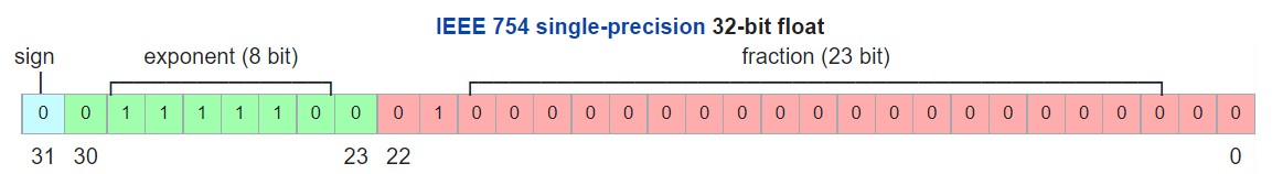
FP32 的表示如下圖
- 1 sign-bit; 8 exponent-bit; 23 fraction-bit (mantissa).
- FP32 normal value 正值範圍: $[3.40 \times10^{-38}, 1.175 \times 10^{+38}]$, 負值範圍乘 (-1).
-
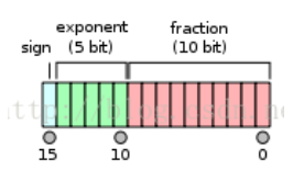
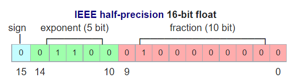
FP16 的表示如下圖:
- 1 sign-bit; 5 exponent-bit; 10 fraction-bit (mantissa).
- FP16 normal and subnormal value 正值範圍: $[5.96\times10^{-8}(\sim 2^{-24} ), 65504 (\sim2^{16})]$, 負值範圍乘 (-1).
-
DLFloat16 (IBM) 如下圖: ARITH_ppt_final_AA (kyoto-u.ac.jp) [@agrawalDLFloat16b2019]
- 1 sign-bit; 6 exponent-bit; 9 fraction-bit (mantissa).
- DLF16 正值範圍: $[4.6\times10^{-10}, 8.59\times10^{+9}]$, 負值範圍乘 (-1).
- BF16 dynamic range 比起 FP16 大很多。 precision 差 6dB? 因爲 mantissa 少了 1-bit: 10-bit -> 9-bit!
- 從 FP16 轉 FP8 容易? 只要把 mantissa 直接砍 16-bit: 23-bit to 7-bit
-
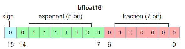
BF16 的表示如下圖:
- 1 sign-bit; 8 exponent-bit; 7 fraction-bit (mantissa).
- BF16 正值範圍: $[1.17\times10^{-38}, 3.39\times10^{+38}]$, 負值範圍乘 (-1).
- BF16 dynamic range 非常大和 FP32 基本一致。但是 precision 並不好,因爲 mantissa 只有 7-bit!
- 從 FP32 轉 FP16 非常容易,只要把 mantissa 直接砍 16-bit: 23-bit to 7-bit
Overflow Problem Statement
考慮 $n$-vectors layer-norm or normalized $l_2$-norm including bias : $\mathbf{x}=\left(x_1, x_2, \ldots, x_n\right) \in \text{FP16}^n$ and a constant bias $\epsilon \in \text{FP16}$, 如何避免計算過程中 overflow 同時保留最大的精度。 \(\begin{align} \|\mathbf{x}\|_2=\sqrt{\frac{1}{n}\sum_{i=1}^n x_i^2 + \epsilon} \end{align}\)
-
這裏假設 $\mathbf{x}$ 是 zero-mean, $\epsilon$ 主要是預防 $|\mathbf{x}|^2_2$ 太小,在後面當做分母造成 overflow. 一般取 $\epsilon \in [+10^{-5} \sim +10^{-4}]$
-
如果 $\mathbf{x}$ 是 zero-mean, 忽略 $\epsilon$ 的影響, $|\mathbf{x}|_2^2$ 其實就是 $\left(x_1, x_2, \ldots, x_n\right)$ 的 variance $= \sigma^2$, $|\mathbf{x}|_2$ 就是 standard deviation $ \sigma$.
-
Caveat: 因爲 $x_1, x_2, …, x_n$ 是正或負,對於 $l_2$-norm 無影響。爲了推導方便,可以假設 $x_1, …, x_n \ge 0$. 如果 $x_i < 0$, 就改成 $-x_i > 0$ 不影響 $l_2$-norm 的計算。
-
FP16 的最大值只有 65504, 計算 $l_2$-norm 過程中的平方項很容易產生 overflow
-
Assumption: Overflow 發生在計算 component 的平方項 $x_k^2$,或是平方和 $\sum_{i=1}^n x_i^2$。最後的 $l_2$-norm 本身不會 overflow (i.e. $\sum_{i=1}^n x_i^2/n > 65504$,但是 $|\mathbf{x}|_2 < 65504$)
Method 1 (with underflow side-effect)
Public Linear Algebra PACKage LAPACK 的做法是 normalized to maximum $x_i$
Let Let $\widehat{x} = \max(x_1, x_2, …, x_n)$ \(\begin{align} \|\mathbf{x}\|_2 = \frac{\widehat{x}}{\sqrt{n}} \times\|\mathbf{x} / \widehat{x}\|_2 \end{align}\) where $\widehat{x}=\max(x_1, x_2, …, x_n)$.
-
這個方法把 normalized $l_2$-norm, $|\mathbf{x} / \widehat{x}|_2$ , 所有的 components 都控制小於等於 1, 避免 overflow. 對於 FP32 沒有問題 ( FP32 的範圍 [$1.4\times 10^{-45}, 3.4\times 10^{38}$] )。
-
但對於 FP16 可能會有 underflow (i.e. $x_k^2 < 5.96\times 10^{-8}$) 造成精度損失的問題。
-
Extreme case: 如果有一個 component 遠大於其他所有 components, i.e. $x_k = \widehat{x} \gg x_i$, 最後的 $l_2$-norm 因爲 underflow 計算結果就會是 $\widehat{x}$, 失去所有其他 component 的 information, i.e. $|\mathbf{x}|_2 = \widehat{x} \times|\mathbf{x} / \widehat{x}|_2 / \sqrt{n} = \widehat{x}/\sqrt{n}$ .
Method 2 (2-segment)
先用簡單的例子説明:
1-dimension: $\mathbf{x}=\left(x_1\right) \text{ including bias } \epsilon\in \text{FP16}$
\[\begin{align*} \|\mathbf{x}\|_2 &=\sqrt{x_1^2 + \epsilon} \end{align*}\]我們可以用 $\beta_H > 0$ 把定義域分成兩段: $x_1 \ge \beta_H$ or $x_1 < \beta_H$. 假設 $\epsilon < \beta_H^2 $.
-
Normal case: $x_1 \le \beta_H$ , 直接計算 $l_2$-norm. 如果 $\beta_H$ 是一個大的 threshold, 大多數情況都是這個 case. For example, $\beta_H = \sqrt{65504} \approx 256$.
-
Special case: $x_1 > \beta_H$, 如果直接計算 $l_2$-norm,在計算 $x_1^2$ 就會 overflow.
此時可以利用 Taylor expansion 避免計算平方項: $\sqrt{1+x} = 1+\frac{x}{2}-\frac{x^2}{8}+\frac{x^3}{16}-\frac{5 x^4}{128}+\frac{7 x^5}{256}+ … = 1+\frac{x}{2}+O(x^2)$
where relative error: $O\left(\frac{\epsilon^2}{x_1^4}\right) \le \frac{\epsilon^2}{\beta_H^4}$ ,
- 選擇 $\beta_H$ 對於 $\epsilon$ ratio 要夠大,才能確保 relative error 夠小。
2-dimension: $\mathbf{x}=\left(x_1, x_2\right) \text{ including bias } \epsilon\in \text{FP16}$.
\[\begin{aligned}\|\mathbf{x}\|_2 &=\sqrt{\frac{x_1^2 + x_2^2}{2} + \epsilon}\end{aligned}\]Let $\widehat{x} = \max(x_1, x_2) > 0$, assuming $\widehat{x} = x_1$
分爲以下 cases:
- Normal case: $\beta_H > \widehat{x}$ :直接計算 $l_2$-norm 不會 overflow. 如果 $\beta_H$ 是一個夠大 threshold, 大部分情況都是這個 case.
- Special case: $\widehat{x} (= x_1) > \beta_H$, 分爲兩種情況
-
$x_1 > \beta_H > x_2$ : 直接計算 $x_1^2$ 會 overflow, 但 $x_2^2$ 不會 overflow
Let $y_1 = \frac{x_1}{\sqrt{2}}$ , $y_2 = \frac{x_2}{\sqrt{2}}$ , and $\epsilon’ = y_2^2 + \epsilon$
顯然上式沒有計算 $x_1^2$ ,不會 overflow!
比較麻煩是下面的情況:
-
$x_1, x_2 > \beta_H$ : 直接計算 $x_1^2$ 或 $x_2^2$ 都會 overflow
Let $K = \sqrt{1 + (\frac{x_2}{\widehat{x}})^2}$ where $ \sqrt{2} > K > 1$ 不會 overflow.
上式沒有計算 $x_1^2$ 或 $x_2^2$, 不會因為平方項 overflow. 因為 $K \le 1 \to $$K \widehat{x} \le \widehat{x} = \max(x_1, x_2)$ 也不會 overflow.
推廣到 n-Dimension $\mathbf{x}=\left(x_1, x_2, …, x_n\right) \text{ including bias } \epsilon\in \text{FP16}$.
Let $\widehat{x} = \max(x_1, x_2, …, x_n)$
- Normal case: $\beta_H > \widehat{x}$ :直接計算 $l_2$-norm 不會 overflow. 如果 $\beta_H$ 是一個夠大 threshold, 大部分情況都是這個 case.
- Special case: $\widehat{x} > \beta_H$
-
可以分成大分量 components: $(x_1, x_2, …, x_m) > \beta_H$ 以及正常分量 components $(x_{m+1}, …, x_n) \le \beta_H $.
Let $K = \sqrt{((\frac{x_1}{\widehat{x}})^2 + … + (\frac{x_m}{\widehat{x}})^2)}$ where $\sqrt{m} \ge K \ge 1$ 不會 overflow (除非 $m \ge 65534^2, 理論上存在,實務不可能$ )
Let $Q = x_{m+1}^2 + … + x_n^2 + n \epsilon$ where $m < n \to S < \beta_H^2$ 不會 overflow, $Q$ 在 $n > 65534$ 有機會 overflow.
可以得到: $K^2 \widehat{x}^2 + Q = \sum_{i=1}^n x_i^2 + n \epsilon = n |\mathbf{x}|_2^2$ , 也就是 $l_2$-norm 的平方。因此 \(\begin{align} \|\mathbf{x}\|_2 &= \sqrt{(x_1^2 + x_2^2 + ... + x_m^2 + x_{m+1}^2 + ...x_n^2)/n + \epsilon} \nonumber\\ &= \sqrt{\frac{K^2 \widehat{x}^2 + Q}{n} } \nonumber\\ &= \frac{K \widehat{x}}{\sqrt{n}} \sqrt{1 + \frac{Q}{K^2 \widehat{x}^2}} \nonumber\\ &\approx \frac{K \widehat{x}}{\sqrt{n}} (1 + \frac{Q }{2 K^2 \widehat{x}^2}) \nonumber\\ &= \frac{1}{\sqrt{n}}(K \widehat{x} + \frac{Q}{2K\widehat{x}}) \label{ndimTaylor} \end{align}\)
Taylor expansion 成立的條件: $K^2 \widehat{x}^2 > Q \to x_1^2 + \ldots +x_m^2 > x_{m+1}^2 + \ldots + x_n^2 + n \epsilon$. 物理上很有意義,就是就是大分量 vector 的 power 必須大於正常分量 vector 的 power. 這個 power ration 值愈大,Taylor expansion 近似就越準確。
定義 $\gamma = \frac{Q}{K \widehat{x}}$ , Taylor expansion 的 error term 大約是 $\gamma^2 / 8$. 如果 $\gamma < 0.3 \,\text{(30\%)}$, 相對誤差大約是 1-2%.
Validate $\eqref{ndimTaylor}$ using 1-dimension and 2-dimension example
1-dimension: $n = 1,\, K=(x_1/x_1)^2 = 1,\, Q = \epsilon \to |\mathbf{x}|_2 = \widehat{x} + \frac{\epsilon}{2\widehat{x}} $ Check!
2-dimension
Special case 1, $n = 2, \, K=1, \, Q=x_2^2 + 2\epsilon \to |\mathbf{x}|_2 = \frac{1}{\sqrt{2}}(\widehat{x} + \frac{x_2^2 + 2 \epsilon}{2\widehat{x}})$ Check!
Special case 2, $n = 2, \, K=\sqrt{1+(x_2/x_1)^2}, \, Q= 2\epsilon \to |\mathbf{x}|_2 = \frac{1}{\sqrt{2}}(K\widehat{x} + \frac{\epsilon}{K \widehat{x}})$ Check!
Overflow Insight and Summary
-
首先計算 $\widehat{x} = \max(x_1, x_2, …, x_n)$: 就是 $\mathbf{x}$ 的最大 component 值。
-
再用 $\beta_H$ 作爲分界綫,如果 $\beta_H > \widehat{x}$ : 屬於 沒有 overflow 的 normal case. 直接計算 $\mathbf{x}$ 的 $l_2$-norm with bias $\epsilon$. (done)
-
如果 $\widehat{x} > \beta_H$ : 屬於 special case. Decompose $\mathbf{x} = (x_1,.., x_m, 0,..,0) + (0, ..,0, x_{m+1}, .., x_n) = \mathbf{x_K} + \mathbf{x_Q}$
where $\mathbf{x_K}$ 所有 non-zero elements 都大於 $\beta_H$ (大分量 vector), and $\mathbf{x_Q}$ 所有 non-zero elements 都小於 $\beta_H$ (正常分量 vector).
-
因此 $|\mathbf{x}|_2^2 = |\mathbf{x}|_K^2 + |\mathbf{x}|_Q^2$, 此處我們把 bias $\epsilon$ 歸在 $\mathbf{x_Q}$ 的 $l_2$ norm; $\mathbf{x_K}$ 的 bias 為 0.
-
因爲 $\mathbf{x_Q}$ 是正常分量 vector, 可以直接計算 $l_2$-norm 的平方 Q (不用開根號),不會 overflow.
-
因爲 $\mathbf{x_K}$ 是大分量 vector, 如果直接計算 $l_2$-norm, 在做平方時會 overflow, 因此需要先 normalize $\mathbf{x_K}$ with $\widehat{x}$. 再計算 normalized vector $\frac{\mathbf{x_K}}{\widehat{x}}$ 的 $l_2$-norm K. 可以避免 overflow,也就是 LAPACK 的方法。 $\mathbf{x_K}$ 的 $l_2$-norm 就是 $K \widehat{x}$ .
-
最後 $\mathbf{x} = \mathbf{x_K} + \mathbf{x_Q}$ 的 $l_2$ norm including bias 就是 $K\widehat{x}$ 加上修正項 $Q/ 2 K\widehat{x}$. (done)
-
-
1-D 和 2-D 的 case 都是 (8) 的特例。
-
(8) 只有在求 $K$ 做一次 element-wise 除法,和一個 scalar 開根號。求 $Q$ 是平方和,不需要開根號。原來的 $l_2$-norm 也需要做平方和,以及一次開根號。
-
Special case approximated $l_2$-norm 比 normal case 的 $l_2$-norm 多了 (i) 一個 (element-wise) max operation; (ii) element-wise comparison with $\beta_H$; (iii) 把原來 vector 拆成兩個 vectors; (iv) 一次 element-wise 除法; (v) 2 個 scalar 乘法,一個 scalar 除法 (除 2 right shift 省略),和一個加法。
Underflow Problem Statement
考慮 $n$-vectors layer-norm or generalized $l_2$-norm including bias : $\mathbf{x}=\left(x_1, x_2, \ldots, x_n\right) \in \text{FP16}^n$ and a constant bias $\epsilon \in \text{FP16}$, 如何避免計算過程中 underflow 造成的精度損失。 \(\begin{aligned} \|\mathbf{x}\|_2=\sqrt{\sum_{i=1}^n x_i^2 + \epsilon} \end{aligned}\)
-
FP16 的最小值只有 $5.96\times 10^{-8}$. 如果 $\mathbf{x}$ 的 component(s) 遠小於 1 但大於最小值, i.e. $5.96\times 10^{-8}<x_i \ll 1$, 在計算 $l_2$-norm 過程中的 component(s) 的平方項很容易產生 underflow (i.e. $x_i^2<5.96\times 10^{-8}$) 影響最後 $l_2$-norm $|\mathbf{x}|_2$ 的精度。 FP32 相對沒有這個問題,因爲 FP32 的最小值為 $1.4\times 10^{-45}$.
- Extreme case: 如果有所有的 components 遠小於 1 但大於最小值, i.e. $5.96\times 10^{-8}<x_i \ll 1$, 同時 components 的平方都 underflow, i.e. $x_i^2 < 5.96\times 10^{-8}$. 最後的 $l_2$-norm 因爲 underflow 計算結果就會是 $\sqrt{\epsilon}$, 失去所有 $\mathbf{x}$ 的 information, i.e. $|\mathbf{x}|_2 = \sqrt{\epsilon}$ .
- Assumption: Underflow 發生在計算的平方項 $x_k^2$ (平方和是 sum of positive number 不會 underflow)。後的 $l_2$-norm 本身不會 underflow (i.e. $x_i^2 < 5.96\times 10^{-8}$,但是 $|\mathbf{x}|2 > 5.96\times 10^{-8}$)。此處暫時不考慮 $\epsilon \approx - \sum{i_i}^n x_i^2$ 所造成的 underflow.
- Caveat: 因爲 $x_1, x_2, …, x_n$ 是正或負,對於 (generalized) $l_2$-norm 無影響。爲了推導方便,可以假設 $x_1, …, x_n \ge 0$. 如果 $x_i < 0$, 就改成 $-x_i > 0$ 不影響 $l_2$-norm 的計算。 Bias $\epsilon$ 可正可負。
Method 1 (help in some case, mostly worse)
Public Linear Algebra PACKage LAPACK 的做法是 normalized to maximum $x_i$.
Let $\widehat{x} = \max(x_1, x_2, …, x_n)$ \(\|\mathbf{x}\|_2 = \widehat{x} \times\|\mathbf{x} / \widehat{x}\|_2\) where $\widehat{x}=\max(x_1, x_2, …, x_n)$.
- normalized $l_2$-norm, $|\mathbf{x} / \widehat{x}|_2$ , 所有的 components 都控制小於等於 1. 對於 FP32 沒有問題 ( FP32 的範圍 [$1.4\times 10^{-45}, 3.4\times 10^{38}$] )。
- 對於 FP16 這個方法只有在所有的 components $x_i$ 都遠小於 1 才有幫助, i.e. $5.96\times 10^{-8}<x_i, \epsilon \ll 1$. 因爲 $\widehat{x}=\max(x_1, …, x_n) < 1$, normalized vector $|\mathbf{x} / \widehat{x}|_2$ 會把所有的 components 放大。不過最大的component 也只放大到 1,只能減輕 underflow.
- (remove) Bias 需要小於 1, i.e. $\epsilon<1$, 不然 bias 放大反而容易造成 overflow, i.e. $\epsilon / \widehat{x} > 65504$.
- 最大的問題是任何一個 $x_i > 1 \to \widehat{x} > 1$, normalized vector $|\mathbf{x} / \widehat{x}|_2$ 會把所有的 components 縮小。只會讓 underflow 問題更 worse.
- 結論: Method 1 在大部分的情況 (any $x_i > 1$),只會讓 underflow 問題更 worse.
Method 2 (2-segment)
先用簡單的例子説明:
1-dimension: $\mathbf{x}=\left(x_1\right) \text{ including bias } \epsilon\in \text{FP16}$
我們可以用 $1 > \beta_L$ 把定義域分成兩段: $x_1 \ge \beta_L$ or $x_1 < \beta_L$.
-
Normal case: $x_1 \ge \beta_L$ , 直接計算 $l_2$-norm. 如果 $\beta_L$ 是一個遠小於 1 的 threshold 但大於等於 FP16 最小精度的平方根,可以避免計算平方時 underflow, i.e. $1 \gg \beta_L > \sqrt{FP16_{min}}$. 大部分情況都是這個 case. 例如我們可以取 $\beta_L = \sqrt{5.96\times 10^{-8}} = 2.4\times 10^{-4}$.
-
Special case: $x_1 < \beta_L \,(2.4\times 10^{-4})$ , 如果直接計算 $l_2$-norm,在計算 $x_1^2$ 就會 underflow. 我們先把上式變形:
到目前爲止都是 exact, 沒有任何近似。對於 non-zero ** $\epsilon \in \text{FP16} \to \sqrt{\epsilon} \in \text{FP16}$ **不會有 underflow. 主要的問題是 $x_1^2 < \beta_L^2$ 會 underflow.
接下來計算判別式:
\(\gamma = \frac{x_1}{\sqrt{\epsilon}}\)
-
如果 $\gamma \ge \beta_L = 2.4\times 10^{-4}$ : 代表 $\epsilon < 1$, $x_i (<\beta_L)$ 除以 $\sqrt{\epsilon}$ 可以放大 $x_1$ 避免 underflow. 可以直接用 (12) 計算 $l_2$-norm 如下: \(\begin{aligned}\|\mathbf{x}\|_2 &=\sqrt{x_1^2 + \epsilon} \\ &= \sqrt{\epsilon} \sqrt{1+ \left(\frac{x_1}{\sqrt{\epsilon}}\right)^2}\\ &= \sqrt{\epsilon} \sqrt{1+ \gamma^2} \end{aligned}\)
-
如果 $\gamma < \beta_L = 2.4\times 10^{-4}$ : 利用 Taylor expansion
\(\begin{aligned}\|\mathbf{x}\|_2 &=\sqrt{x_1^2 + \epsilon} \\ &= \sqrt{\epsilon} \sqrt{1+ \left(\frac{x_1}{\sqrt{\epsilon}}\right)^2}\\ &= \sqrt{\epsilon} \sqrt{1+ \gamma^2} \\ & \approx \sqrt{\epsilon} (1+ \frac{\gamma^2}{2}) = \sqrt{\epsilon} + \frac{(\sqrt{\epsilon}\gamma)\gamma}{2} \end{aligned}\) 除非 $\epsilon > 1$, $\sqrt{\epsilon} \gamma $ 可以把 $\gamma$ 放大到 underflow threshold 以上,不然第二 (修正) 項在 FP16 dynamic range 無法 cover.
#### n-Dimension $\mathbf{x}=\left(x_1, x_2, …, x_n\right) \text{ including bias } \epsilon\in \text{FP16}$.
Let $x_{min} = \min(x_1, x_2, …, x_n)$
我們可以用 $1 > \beta_L > 0$ 把定義域分成兩段: $x_1 \ge \beta_L$ or $x_1 < \beta_L$.
- Normal case: $x_{min} \ge \beta_L$ , 直接計算 $l_2$-norm. 如果 $\beta_L$ 是一個遠小於 1 的 threshold $1 \gg \beta_L$, 大部分情況都是這個 case. For example, $\beta_L = \sqrt{5.96\times 10^{-8}} = 2.4\times 10^{-4}$.
- Special case: $x_{min} < \beta_L$
-
可以分成小分量 components: $(x_1, x_2, …, x_m) < \beta_L$ 以及正常分量 components $(x_{m+1}, …, x_n) \ge \beta_L $.
Let $K^2 = (\frac{x_1}{\tilde{x}})^2 + … + (\frac{x_m}{\tilde{x}})^2$ where $\tilde{x} = \max(x_1, .., x_m)$
Let $Q^2 = x_{m+1}^2 + … + x_n^2 + \epsilon$
-
Caveat 1: $\tilde{x} < \beta_L = 2.4\times 10^{-4}$ and $\sqrt{m} > K > 1$
-
Caveat 2: $Q > (n-m+1) \beta_L + \epsilon $
可以得到: $K^2 \tilde{x}^2 + Q^2 = \sum_{i=1}^n x_i^2 + \epsilon = |\mathbf{x}|_2^2$ , 也就是 $l_2$-norm 的平方。因此
到目前爲止都是 exact, 沒有任何近似。$K>1$ 不會有 underflow 問題。$Q$ 是正常分量的 $l_2$-norm, 也沒有 underflow 的問題。唯一的問題是 $\tilde{x}^2 < \beta_L^2 = 5.96\times 10^{-8}$ 會有 underflow 的問題。
接下來計算判別式:
\(\gamma = \frac{K\tilde{x}}{Q}\)
-
如果 $\gamma > \beta_L = 2.4\times 10^{-4}$, 直接利用 (16) 計算 $|\mathbf{x}|_2 $ 如下式。不會有 underflow 問題, done. \(\begin{aligned}\|\mathbf{x}\|_2 &=\sqrt{x_1^2 + x_2^2 + ... + x_m^2 + x_{m+1}^2 + ...x_n^2 + \epsilon} \\&= \sqrt{K^2 \tilde{x}^2 + Q^2} \\&= Q \sqrt{1 + \frac{K^2\tilde{x}^2}{Q^2}} \\ &= Q \sqrt{1+\gamma^2} \end{aligned}\)
-
如果 $\gamma \le \beta_L = 2.4\times 10^{-4}$, 利用 Taylor expansion again:
如果 $Q > 1$, 就是利用 $Q$ 把 $\gamma$ 放大,避免 underflow 的問題。如果 $Q < 1$, 代表小分量無法用 FP16 精度表示, done.
### Underflow Insight and Summary
-
首先計算 $x_{min} = \min(x_1, x_2, …, x_n)$: 就是 $\mathbf{x}$ 的最小 component 值。
-
再用 $\beta_L$ 作爲分界綫,如果 $x_{min} \ge \beta_L$ : 屬於沒有 underflow 的 normal case. 直接計算 $\mathbf{x}$ 的 $l_2$-norm with bias $\epsilon$. (done)
-
如果 $x_{min} < \beta_L$ : 屬於 special case. Decompose $\mathbf{x} = (x_1,.., x_m, 0,..,0) + (0, ..,0, x_{m+1}, .., x_n) = \mathbf{x_K} + \mathbf{x_Q}$
where $\mathbf{x_K}$ 所有 non-zero elements 都小於 $\beta_L$ (小分量 vector), and $\mathbf{x_Q}$ 所有 non-zero elements 都大於 $\beta_H$ (正常分量 vector). 此時要多做一個 $\mathbf{x_K}$ 的 max: $\tilde{x} = \max(x_1, .., x_m, 0, ..0)$
- 因此 $|\mathbf{x}|_2^2 = |\mathbf{x}|_K^2 + |\mathbf{x}|_Q^2$, 此處我們把 bias $\epsilon$ 歸在 $\mathbf{x_Q}$ 的 $l_2$ norm; $\mathbf{x_K}$ 的 bias 為 0.
- 因爲 $\mathbf{x_Q}$ 是正常分量 vector, 可以直接計算 $l_2$-norm Q,不會 underflow.
- 因爲 $\mathbf{x_K}$ 是小分量 vector, 如果直接計算 $l_2$-norm, 在做平方時會 underflow, 因此需要先 normalize $\mathbf{x_K}$ with $\tilde{x}$. 再計算 normalized vector $\frac{\mathbf{x_K}}{\tilde{x}}$ 的 $l_2$-norm K, 可以避免 underflow. $\mathbf{x_K}$ 的 $l_2$-norm 就是 $K \tilde{x}$ .
- 計算判別式 $\gamma = \frac{K\tilde{x}}{Q}$ , 如果 $\gamma > \beta_L$, $|\mathbf{x}|_2 = Q \sqrt{1+\gamma^2}$ 沒有 underflow (done)
- 如果 $\gamma < \beta_L$, 利用 Taylor expansion: $|\mathbf{x}|_2 = Q + (Q\gamma)\gamma/2$ (done)
-
Special case $l_2$-norm 比 normal case 的 $l_2$-norm 多了 (i) 一個 (element-wise) min 和一個max operation; (ii) element-wise comparison with $\beta_L$; (iii) 把原來 vector 拆成兩個 vectors; (iv) 一次 element-wise 除法; (v) 還有幾個 scalar 乘法,除法,和開根號。
推廣到 n-Dimension $\mathbf{x}=\left(x_1, x_2, …, x_n\right) \text{ including bias } \epsilon\in \text{FP16}$.
Let $\widehat{x} = \max(x_1, x_2, …, x_n)$
- Normal case: $\beta_H > \widehat{x}$ :直接計算 $l_2$-norm 不會 overflow. 如果 $\beta_H$ 是一個夠大 threshold, 大部分情況都是這個 case.
- Special case: $\widehat{x} > \beta_H$
-
可以分成大分量 components: $(x_1, x_2, …, x_m) > \beta_H$ 以及正常分量 components $(x_{m+1}, …, x_n) \le \beta_H $.
Let $K = \sqrt{((\frac{x_1}{\widehat{x}})^2 + … + (\frac{x_m}{\widehat{x}})^2)/m}$ where $K \le 1$ 不會 overflow
Let $n Q^2 = x_{m+1}^2 + … + x_n^2 + n \epsilon$ ($m < n$, 一般 $m \ll n$) where $Q < \beta_H$ 不會 overflow
可以得到: $K^2 m \widehat{x}^2 + Q^2 = \sum_{i=1}^n x_i^2 + n \epsilon = n |\mathbf{x}|_2^2$ , 也就是 $l_2$-norm 的平方。因此 \(\begin{aligned}\|\mathbf{x}\|_2 &= \sqrt{(x_1^2 + x_2^2 + ... + x_m^2 + x_{m+1}^2 + ...x_n^2)/n + \epsilon} \\ &= \sqrt{\frac{m K^2 \widehat{x}^2 + n Q^2}{n} } \\ &= K \widehat{x} \sqrt{1 + \frac{n Q^2}{m K^2 \widehat{x}^2}} \sqrt{\frac{m}{n}}\\ &\approx K \widehat{x} (1 + \frac{n Q^2 }{2 m K^2 \widehat{x}^2})\sqrt{\frac{m}{n}}\\ &= K \widehat{x} \sqrt{\frac{m}{n}} + \frac{Q^2}{2K\widehat{x}}\sqrt{\frac{n}{m}} \end{aligned}\)
where $Q^2 < \beta_H^2, m K^2 \widehat{x}^2 > m \beta_H^2$, 所以 Taylor series 會收斂。
Check special case 1-D: m = 1, n = 1 : $Q^2 = \epsilon$ and $K=(x_1/x_1)^2 = 1 \to |\mathbf{x}|_2 = \widehat{x} + \frac{\epsilon}{2\widehat{x}} $ Yes!
Check special case 2-D (a): m = 1, n = 2 : $K^2 = (x_1/x_1)^2 = 1 \to K = 1$
$2 Q^2 = x_2^2 + 2 \epsilon \to Q^2 = x_2^2/2 + \epsilon$
$|\mathbf{x}|_2 = \frac{\widehat{x}}{\sqrt{2}} + \sqrt{2}\frac{x_2^2/2+\epsilon}{2 \widehat{x}} = \frac{1}{\sqrt{2}}(\widehat{x}+\frac{x_2^2 + 2\epsilon}{2\widehat{x}}) $ Yes!
Check special case 2-D (b): m = 2, n = 2 : $2 K^2 = (x_1/x_1)^2 + (x_2/x_1)^2 = 1 + (x_2/x_1)^2 $, and $Q^2 = \epsilon$
$|\mathbf{x}|_2 = K {\widehat{x}} + \frac{\epsilon}{2 K \widehat{x}}$ Yes!
Is is better to choose? : $\sqrt{n} Q’^2 = x_{m+1}^2 + … + x_n^2 + n \epsilon \to \sqrt{n} Q’^2 = n Q^2 \to \sqrt{n} Q^2 = Q’^2$
therefore: \(\begin{aligned}\|\mathbf{x}\|_2 &\approx K \widehat{x} \sqrt{\frac{m}{n}} + \frac{Q^2}{2K\widehat{x}}\sqrt{\frac{n}{m}} \\ &= K \widehat{x} \sqrt{\frac{m}{n}} + \frac{Q'^2}{2K\widehat{x}\sqrt{m}} \end{aligned}\)
####
Further task:
-
Reduce computation complexity
-
multiply by power of 2, divide by power of 2, the constant can be arbitrary value
-
catch: Kx_bar, 所以可以是 2^power, no need to be max. => task!
-
-
Other format:
- FP8, BF16, DLF16, etc.
- DFL16, FP8 different format, beta and scaling factor
- parameter choose is very interesting!
-
Improve the flexibility (for FP8, …)
- Assuming sign-bit can be used because of norm is positive (change neg to pos)
-
How about scaler multiplication use FP32? to solve the problem once for all!
- 如果讓 scalar (not vector) engine support FP32, 是否有好處?
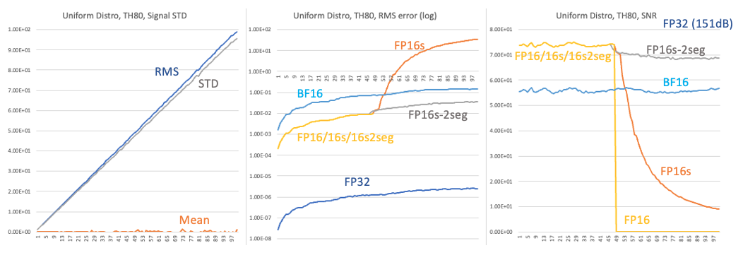
FP16/FP16S (saturation) vs. FP16S 2-segment vs. BF16 performance
Uniform distribution (vector length = 16), internal accumulator FP16S
-
上圖左 is uniform distribution: std = [1: 100], Mean (orange), STD (grey), RMS (blue): $\sigma^2 = \text{RMS}^2 - \overline{x}^2 $. 我們用 RMS 作為計算 SNR 的 signal power. STD 和 RMS 的誤差可以忽略不計。
-
上圖中是 error 圖。為了看得清楚,y-axis 使用 log-scale.
- Caveat: uniform distribution STD = (b-a)/sqrt(12) let b = range and a = -range => range = STD * sqrt(3).
- FP32 顯然有最小的 RMS error, no surprise.
- FP16/16s/16s2seg 在 STD < 47 基本都一樣,no surprise. 但在 STD > 48 表現完全不同。
- FP16 在 STD > 48 overflow, error 變成無限大。Why?
- STD = 48 對應的 uniform distribution range 就是 [-83-83].
- FP16_MAX = 65504, 平方項的 overflow limit 是 sqrt(65504) = 255.9 or 256.
-
256/83 = 3, any insight?
- 因為 Threshold = 80 => STD = 80/sqrt((3)) = 46. 所以 STD 在 48 之後就爆棚。
- 為什麼 Threshold 80
- 為什麼是 STD > 48 error 上升? 因為 FP16 input signal 超過 80 threshold = 80, 80 / sqrt(3)
- FP16_MAX = 65504. 因為是 vector length = 16. 所以 sqrt(65504) = 256 -> 256/16 = 16.
https://tex.stackexchange.com/questions/416450/the-formula-alignment-across-a-table-column
1 | |
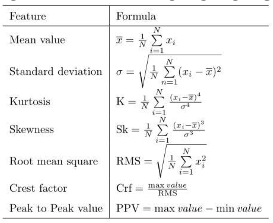
\(\text{Mean value} & \overline{x}=\frac{1}{N}\sum_{i=1}^{N}x_i \\
\text{Standard deviation} & \sigma = \sqrt{\frac{1}{N}\sum_{n=1}^{N}(x_i - \overline{x})^2} \\
\text{Kurtosis} & \text{K}=\frac{1}{N}\sum_{i=1}^{N}\frac{(x_i-\overline{x})^4}{\sigma^4} \\
\text{Skewness} & \text{Sk} = \frac{1}{N}\sum_{i=1}^{N}\frac{(x_i-\overline{x})^3}{\sigma^3} \\
\text{Root mean square} & \text{RMS} = \sqrt{\frac{1}{N}\sum_{i=1}^{N}x_i^{2}} \\
\text{Crest factor} & \text{Crf} = \frac{\max \text{value}}{\text{RMS}} \\
\text{Peak to Peak value} & \text{PPV} = \max \text{value} - \min \text{value}\)
容易證明 $\sigma^2 = \text{RMS}^2 - \overline{x}^2 $