Reference
-
https://blog.csdn.net/qq_34554039/article/details/122087189
-
https://blog.csdn.net/wxc971231/article/details/124629256
Softmax
Softmax 數學定義
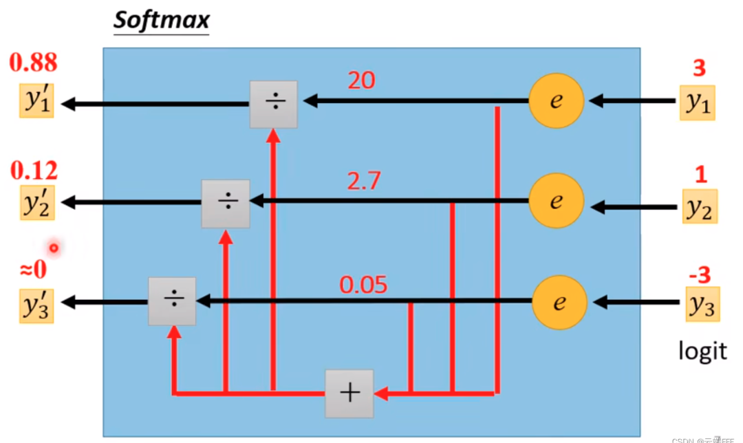
\[\operatorname{softmax}\left(x_i\right)=\frac{\exp \left(x_i\right)}{\sum_j^n \exp \left(x_i\right)}\]分子經過 exponent operation 轉換為正值,同時保留順序。比較麻煩的是分母,需要加總所有的 exponent terms 作為 normallization constant. 可是偏偏又要計算。
Softmax 的作用是把 input values 轉換成 probability (between 0 and 1), 同時保持原來的大小順序。
廣泛用於 CNN 最後的分類。在 transformer 也是非常重要的算子。
為什麼 softmax 重要? Pro:
- 不論正負 input values 多大的 dynamic range, Output 都可以轉換為 positive between [0, 1] 之間的機率,總和為 1.
- Output 有清晰的物理意義 (機率)。可以連接 deterministics values to probability (Bayesian) interpretation.
-
連續可微分。back-propagation 非常容易。
-
Con:
- Exponent 運算容易 overflow. Normalization factor 非常繁瑣。
Overflow Problem Statement
考慮 $n$-vectors softmax: $\mathbf{x}=\left(x_1, x_2, \ldots, x_n\right) \in \text{FP16}^n$ and a constant bias $\epsilon \in \text{FP16}$, 如何避免計算過程中 overflow 同時保留最大的精度。
\[\operatorname{softmax}\left(x_i\right)=\frac{\exp \left(x_i\right)}{\sum_{i=1}^n \exp \left(x_i\right) + \epsilon}\]-
$\epsilon$ 主要是預防 $\sum_{i=1}^n \exp \left(x_i\right)$ 太小,在分母 underflow to 0 造成 divide 0 error, 一般取 $\epsilon \in [+10^{-5} \sim +10^{-4}]$
-
FP16 的最大值只有 65504, 計算 $\exp(x_i)$ 或是 $\sum_{i=1}^n \exp \left(x_i\right)$ 過程中很容易產生 overflow.
-
Assumption: $x_i \ll 65504$, overflow 發生在計算 $\exp(x_i)$ 或是和, e.g. $\exp(12) = 162754 > 65504$。最後的 softmax in [0, 1] 不會 overflow (of course).
如何避免 Softmax Overflow
Method 1: Normalization
- 找到向量 $\boldsymbol{x}$ 中的最大值:
- softmax的分子、分母同时除以c
经过上述变换, 分子的最大取值变为了 $\exp (0)=1$, 避免 overflow; 分母中至少会 $+1$, 避免了分母为 0 造成 underflow 除 0。 \(\begin{aligned} \sum_j^n \exp \left(x_j-c\right) &=\exp \left(x_i-c\right)+\exp \left(x_2-c\right)+\ldots+\exp \left(x_{\max }-c\right) \\ =& \exp \left(x_1-c\right)+\exp \left(x_2-c\right)+\ldots+1 \end{aligned}\)
- Pro: 同時解決 overflow and underflow problems
-
Con: 浪費了 floating point 大於 1 部分的 dynamic range, 15 個 octaves.
-
一個方法是 select c such that $\exp(x_{max} - c)$ 落在 FP16 max, 也就是 $x_{max} - c < \ln(65504) = 11 \to c = x_{max} - 11$ 附近, instead of $x_{max} - c = 0 \to c = x_{max}$ 。如此可以最大保留 dynamic range for softmax!
- 不過看起來好像也只有增加 11 的 dynamic range 因為 $\exp$ 膨脹太快。是否有更好的方法?
Bias = 0
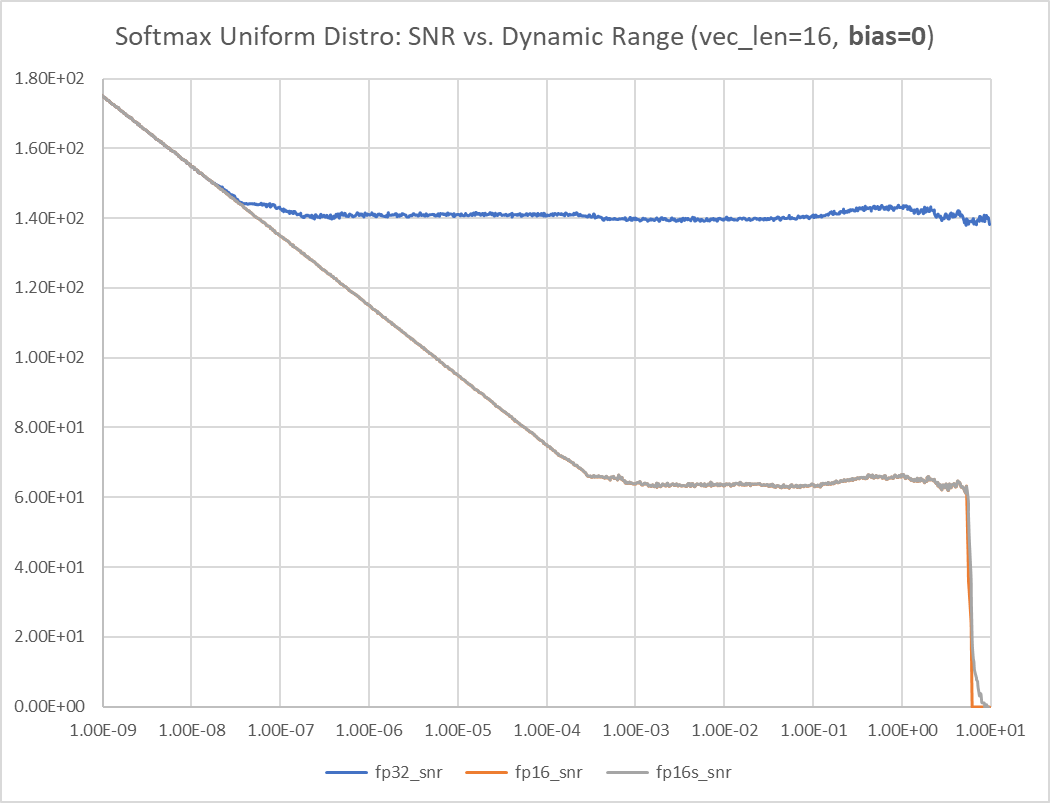
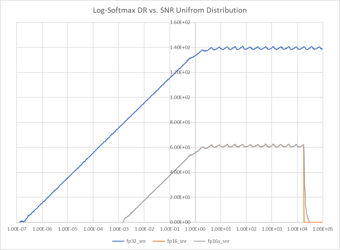
- SNR: signal is the max(softmax(xi)), noise is the max( softmax(xi)-golden softmax(xi))
- 在平坦區 SNR FP32 = 142dB. FP16 = 66dB
- For FP16 and FP16s (no much difference), the threshold is around sigma = 5.3, the uniform distribution is between [-5.3sqrt(3), +5.3sqrt(3)] = [-9.2, +9.2], vector length = 16, nan threshold is 11, 11/9.2 = 1.2
- 不過有誤解在 signal 很小 SNR 很大!!! 因爲 signal 很小, max(softmax(xi) = softmax(x0) = softmax(x1) == softmax(x15) = 0.0625. 因爲 noise 很小,所以 SNR 很大。
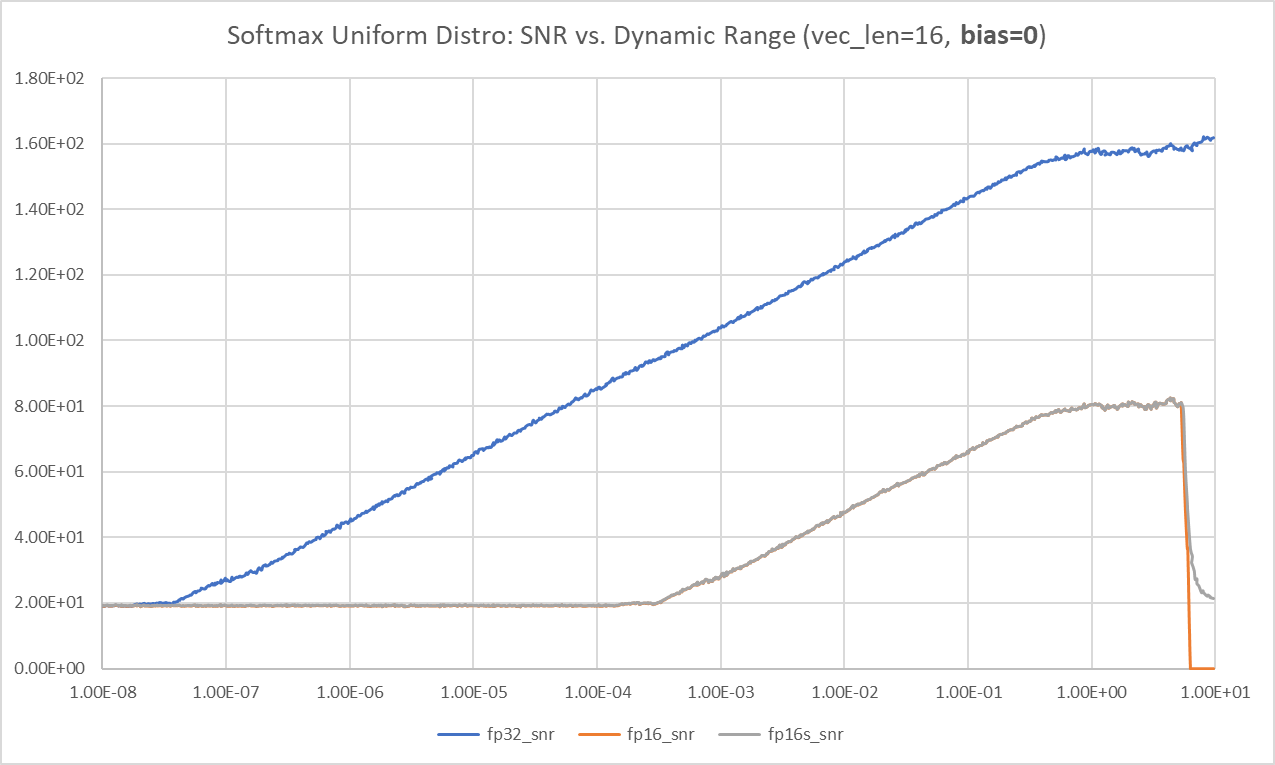
- 顯然不合理,So I change to use input power as signal!! i.e. std(xi). 這樣合理多了。
- but why there is a 20dB noise floor at very small signal?
- 在平坦區 SNR FP32 = 158dB. FP16 = 80dB
- 所以 bias=0 for FP16 dynamic range is only at 5.3
- The dynamic range is very narrow when bias = 0, only 1 decade? [0.5, 5.7] = 3.5 octaves.
Bias = max(xi)
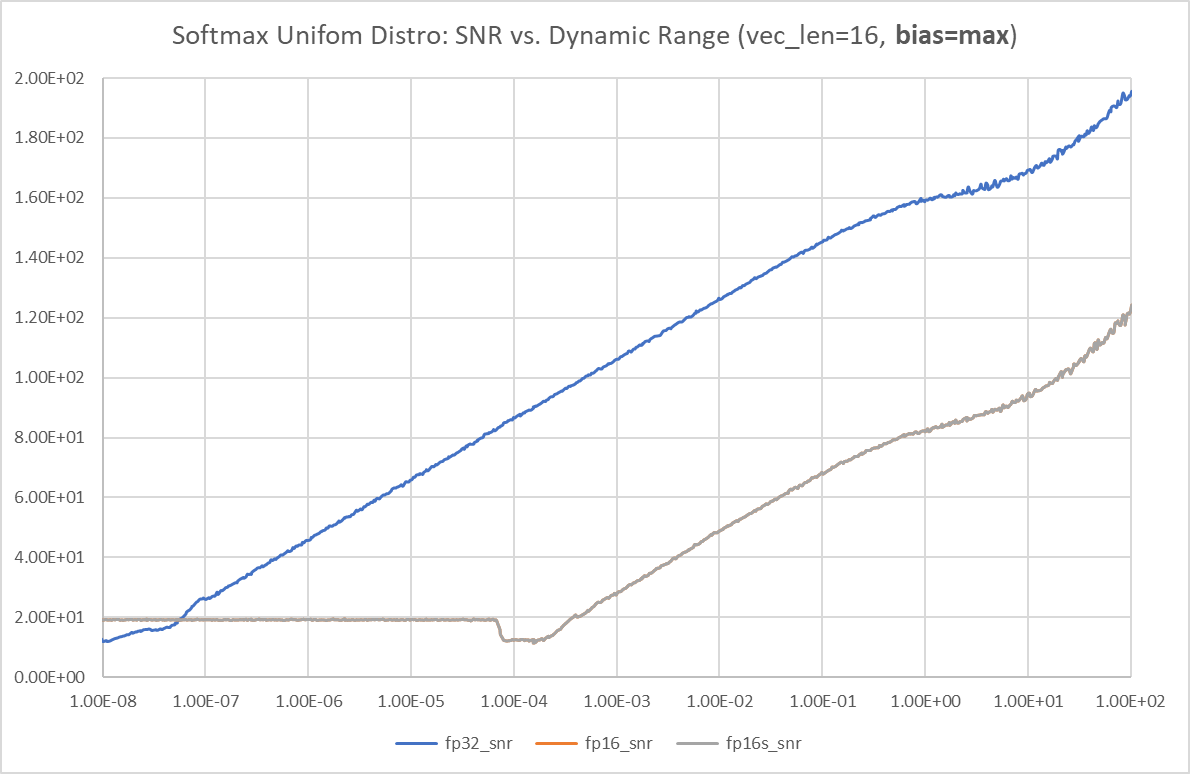
FP16 沒有 max dynamic range 的問題。但是 softmax 的 output 接近 1, 所以 noise is compressed and the SNR keeps increase (假的)。要同時看 softmax 的 dynamic range!
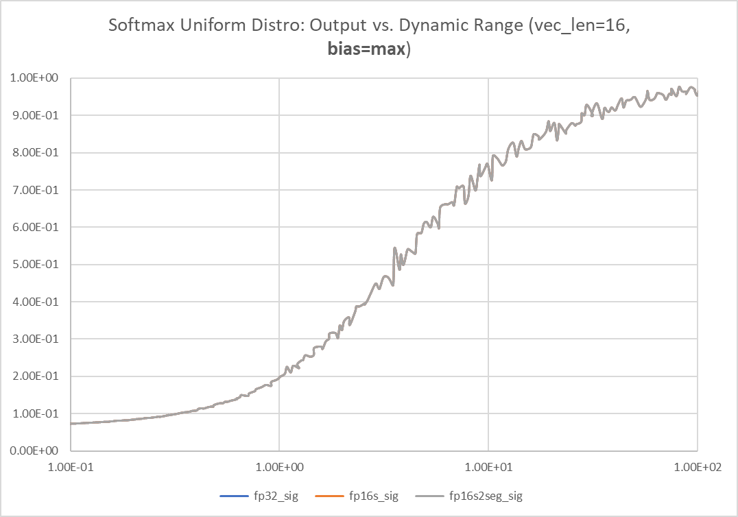
因爲當 leading signal 接近 1, 很難判斷 error, 因爲都被 compress to 1. 試著用 log exp sum. Looks very good!
How to Shift the Dynamic Range?
use the bias !!
How to expand the dynamic range (or contract the dynamic range? and trade-off the SNR?)
Method 2: Log-Sum_Exp Trick
要壓制 $\exp$ 膨脹的問題,直觀就是取 $\log_e = \log$, 這裡 log 是用 e base.
Pro:
- 避免 underflow 对数运算可以将相乘变为相加, 即: $\log \left(\mathrm{x}_1 \mathrm{x}_2\right)=\log \left(\mathrm{x}_1\right)+\log \left(\mathrm{x}_2\right)$ 。当两个很小的数 $\mathrm{x}_1 、 \mathrm{x}_2$ 相 乘时, 其乘积会变得更小, 超出精度则下溢出; 而对数操作将乘积变为相加, 降低了 underflow 的风险。除法變成減法沒有除 0 的問題。
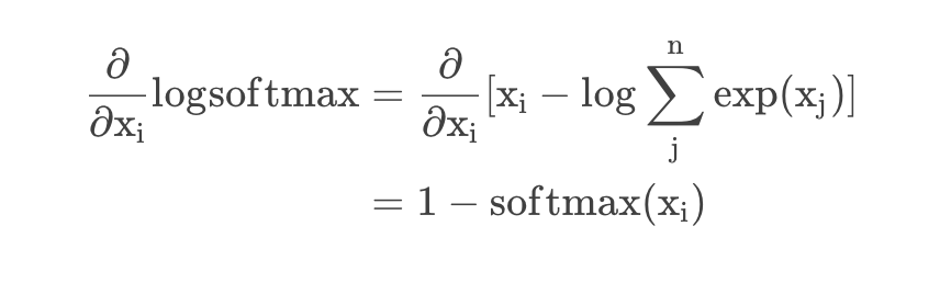
- 避免 overflow $\log \operatorname{-softmax}$ 的定义: \(\begin{aligned} \log\operatorname{-softmax} &=\log \left[\operatorname{softmax}(x_i)\right] \\ &=\log \left(\frac{\exp \left(x_i\right)}{\sum_{j=1}^{n} \exp \left(x_j\right)}\right) \\ &=x_i - \log \left[\sum_{j=1}^{n} \exp \left(x_j\right)\right] \end{aligned}\) 令 $y=\log \sum_{j=1}^{n} \exp (x_j)$, 当 $x_j$ 的取值过大时, $y$ 存在 overflow 的风险, 因此, 采用与3.3中同样的Trick: \(\begin{aligned} y &=\log \sum_{j=1}^{n} \exp \left(x_j\right) \\ &=\log \sum_{\mathrm{j}}^{\mathrm{n}} \exp \left(\mathrm{x}_{\mathrm{j}}-\mathrm{c}\right) \exp (\mathrm{c}) \\ &=\mathrm{c}+\log \sum_{\mathrm{j}}^{\mathrm{n}} \exp \left(\mathrm{x}_{\mathrm{j}}-\mathrm{c}\right) \end{aligned}\) 当 $c=\max (\boldsymbol{x})$ 时,可避免上溢出。 此时, $\log\operatorname{-softmax}$ 的计算公式变为: (其实等价于直接对 $3.3$ 节的Trick取对数) \(\log \operatorname{-softmax}=\left(x_i-c\right)-\log \sum_j^n \exp \left(x_j-c\right)\) Con
這樣看起來好像也沒有好處:overflow 的條件和之前一樣,還要多算一個 log, 以及最後要多一個 exp 才能得到 softmax!
Softmax Related Math
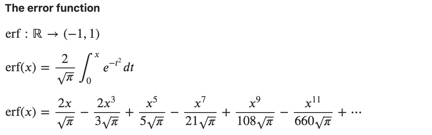
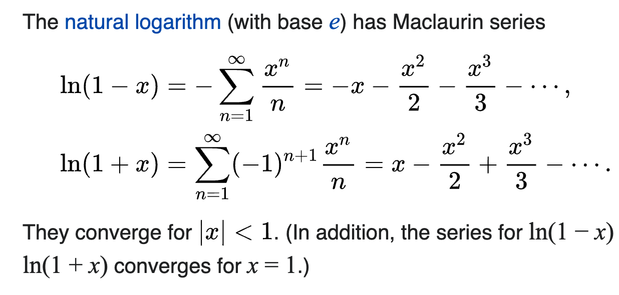
Eq.1: Taylor series of $\ln x$ at an arbitrary nonzero point $a$ is: \(\ln a+\frac{1}{a}(x-a)-\frac{1}{a^2} \frac{(x-a)^2}{2}+\cdots .\) The natural logarithm (with base $e$ ) has Maclaurin series \(\begin{aligned} &\ln (1-x)=-\sum_{n=1}^{\infty} \frac{x^n}{n}=-x-\frac{x^2}{2}-\frac{x^3}{3}-\cdots \\ &\ln (1+x)=\sum_{n=1}^{\infty}(-1)^{n+1} \frac{x^n}{n}=x-\frac{x^2}{2}+\frac{x^3}{3}-\cdots \end{aligned}\) They converge for $|x|<1$. In addition, the series for $\ln (1-x)$ and $\ln (1+x)$ converges for $x=1$. 不過收斂很慢。
Eq.2: The Maclaurin series of the exponential function $e^x$ is \(\begin{aligned} e^x = \sum_{n=0}^{\infty} \frac{x^n}{n !} &=\frac{x^0}{0 !}+\frac{x^1}{1 !}+\frac{x^2}{2 !}+\frac{x^3}{3 !}+\frac{x^4}{4 !}+\frac{x^5}{5 !}+\cdots \\ &=1+x+\frac{x^2}{2}+\frac{x^3}{6}+\frac{x^4}{24}+\frac{x^5}{120}+\cdots \end{aligned}\) 以上的 Taylor expansion 對於任何 $x$ 都收斂,因為分母的 factor function 後來會增加非常快,遠遠超過任何 polynomial growth, i.e. $n! \gg x^n$, when $n$ is large.
| 不過如果求近似解,最好是 $ | x | <1$ 才收斂快。 |
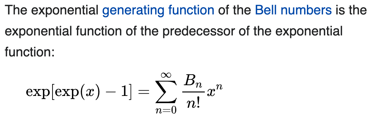
Eq.2b: The exponential generating function of the Bell numbers: \(e^{e^x -1} = \sum_{n=0}^{\infty} \frac{B_n}{n !} x^n\)
可以應用在幾個常見的 functions:
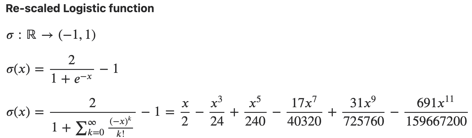
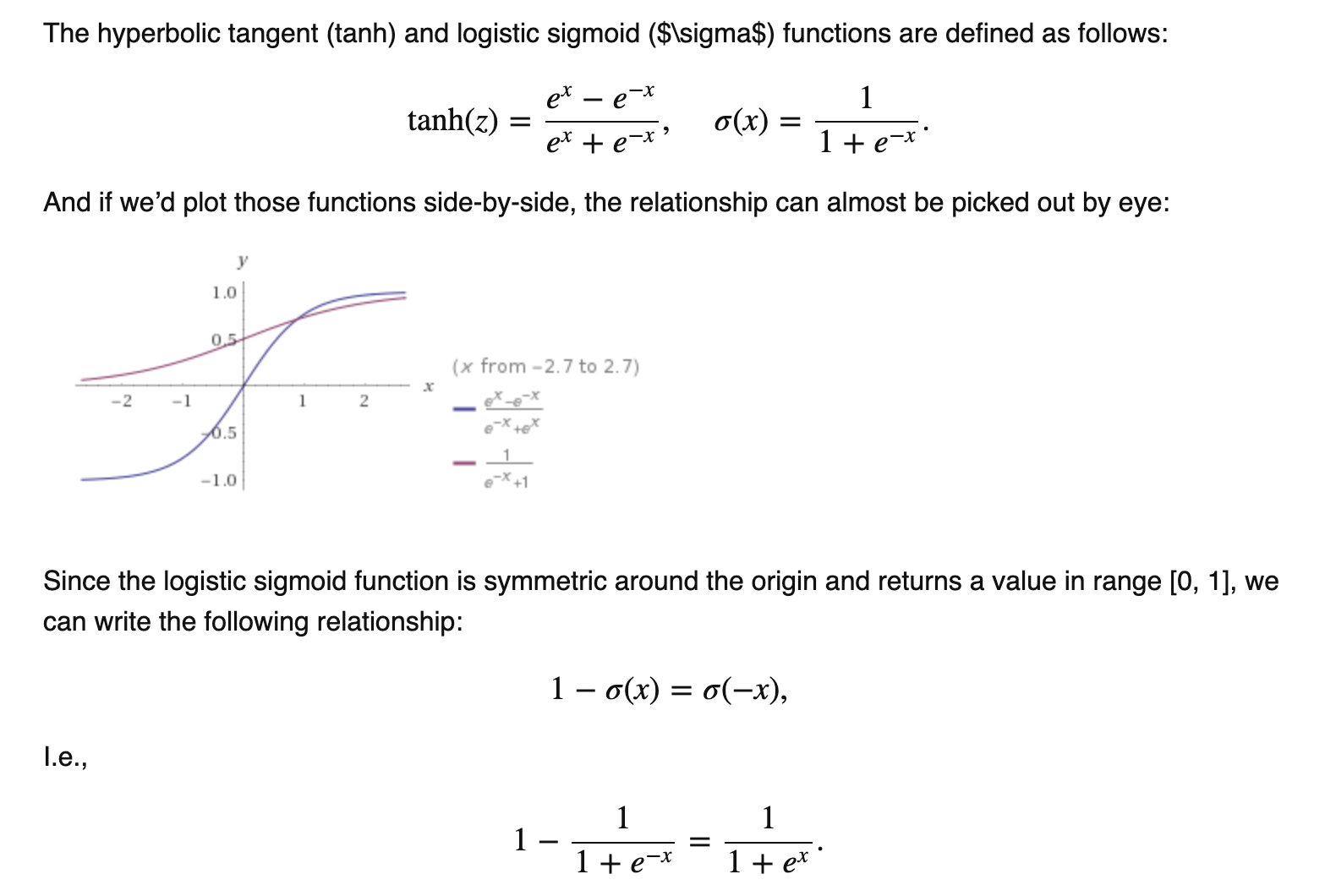
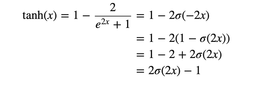
\[\sinh x &= \frac{e^{x} - e^{-x}}{2} \sim x + \frac{x^3}{6} + o(x^5)\\ \cosh x &= \frac{e^{x} + e^{-x}}{2} \sim 1 + \frac{x^2}{2} + o(x^4) \\ \tanh x &= \frac{\sinh x}{\cosh x} = \frac{e^x - e^{-x}}{e^x + e^{-x}} \sim x - \frac{x^3}{3} + o(x^5) \\\] \[\tanh x=\sum_{n=1}^{\infty} \frac{B_{2 n} 4^n\left(4^n-1\right)}{(2 n) !} x^{2 n-1} \quad=x-\frac{x^3}{3}+\frac{2 x^5}{15}-\frac{17 x^7}{315}+\cdots \quad \text { for }|x|<\frac{\pi}{2}\]Caveat: logsitic function 和 tanh function 有直接的關係如下。
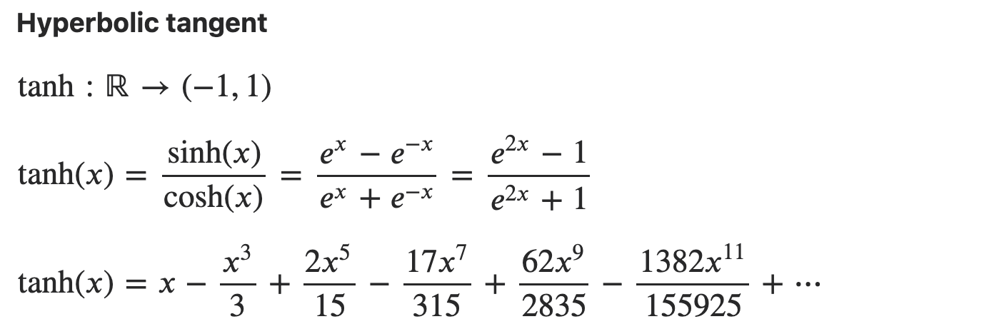
看起來收斂的速度不錯,只要前兩項就可以讓 error 到 $x^5$ 項。不過收斂的範圍有點小。
如果只取前兩項, tanh = x - x^3/3 = -x(x-a)(x+a)
(Only when 0<x<a) 如果再用 log tanh = log x + log (a-x) + log (a+x)
只要是 odd function 都有這個機會。
f(x) = f(-x). f(x) ~ x - a x^3 + … =>. f(x) ~ x - a x^3 = - x (x-a)(x+a), error ~ x^5
如果要用在 logistic function 或是 softmax function 會有困難,因為兩者都不是 odd function.
不過還是有機會讓 f(x) = x + a x^2 + b x^3, error ~ x^4 => -x (x+a)(x+b)
How?
log (1+e^{-x}) =


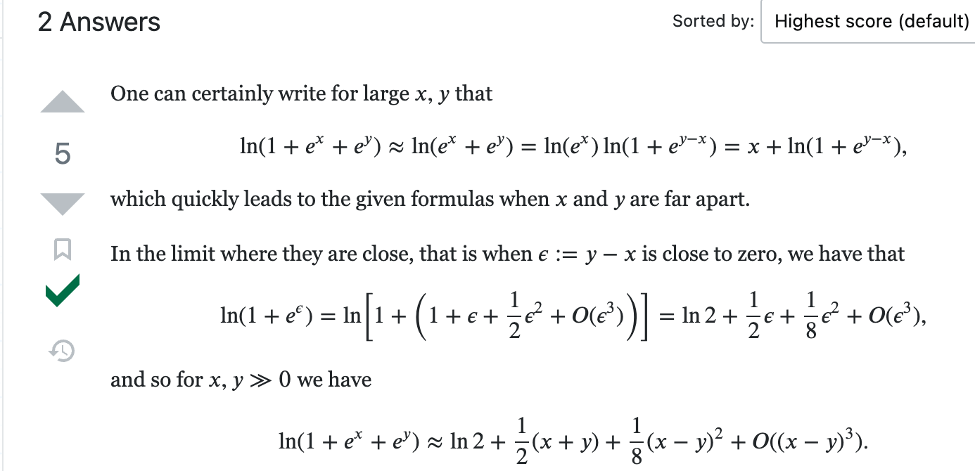
https://math.stackexchange.com/questions/1177841/approximating-ln1-expx-expy
https://stackoverflow.com/questions/62767438/expand-1-dim-vector-by-using-taylor-series-of-log1ex-in-python. : very good discussion.
**Eq.3a: $\log (e^{x}-1)$ and $\log (1 - e^{-x})$ for $x>0$ **
https://zhuanlan.zhihu.com/p/28037156
顯然只有在 $x > 0$ 才有意義。
-
注意 $\log (e^{x}-1) = x + \log(1-e^{-x})$, 所以只要看 $\log(1-e^{-x})$ 即可。
-
$x\to 0^+ \Rightarrow 1-e^{-x} \to 0^+ \Rightarrow \log(1-e^{-x}) \to -\infty$
-
$x \to +\infty \Rightarrow e^{-x} \to 0^+ \Rightarrow \log(1-e^{-x})\to 0^-$
- 因為這兩個部分都有數值 inaccurate 問題,因此有兩個近似:
-
expm1 = $e^x - 1$ for $x\to 0^+$ \(\begin{aligned} e^x - 1 = \sum_{n=1}^{\infty} \frac{x^n}{n !} &=x+\frac{x^2}{2 !}+\frac{x^3}{3 !}+\frac{x^4}{4 !}+\frac{x^5}{5 !}+\cdots \\ &=x+\frac{x^2}{2}+\frac{x^3}{6}+\frac{x^4}{24}+\frac{x^5}{120}+\cdots \end{aligned}\)
\[\begin{aligned} 1-e^{-x} &= x -\frac{x^2}{2 !}+\frac{x^3}{3 !}-\frac{x^4}{4 !}+\frac{x^5}{5 !}+\cdots \end{aligned}\]$\lim_{x\to 0^+}\log (1 - e^{-x}) = \lim_{x\to 0^+}\log(x-\frac{x^2}{2!}+…) \sim \lim_{x\to 0+}\log x (\to -\infty)$
$\lim_{x\to 0^-}\log (1 - e^{x}) = \lim_{x\to 0^-}\log(-x-\frac{x^2}{2!}-…) \sim \lim_{x\to 0^-}\log (-x) (\to -\infty)$
-
log1p $= \log (1+y) = y -\frac{y^2}{2}+\frac{y^3}{3}-\frac{y^4}{4}+\frac{y^5}{5}-\cdots$
Let $y = -e^{-x}$
\[\begin{aligned} \lim_{x\to \infty}\log (1-e^{-x}) = \lim_{x\to \infty}(-e^{-x} - \frac{e^{-2x}}{2} - ...) \sim \lim_{x\to \infty} -e^{-x} (\to 0^-) \end{aligned}\] \[\begin{aligned} \lim_{x\to -\infty}\log (1-e^{x}) = \lim_{x\to -\infty}(-e^{x} - \frac{e^{2x}}{2} - ...) \sim \lim_{x\to -\infty} -e^{x} (\to 0^-) \end{aligned}\]
-
-
什麽時候用 expm1 和 log1p? 根據 reference:
- $x > \log 2$ 使用 log1p: $\log (1-e^{-x}) = \text{log1p}(-e^{-x})$ or $\log (e^x-1) = x + \text{log1p}(-e^{-x})$
- $x < \log 2$ 使用 expm1: $\log (1-e^{-x}) = \log (- \text{expm1}(-x)) $ or $\log (e^x-1) = \log (\text{expm1}(x)) = x + \log (- \text{expm1}(-x))$
 {
{
Eq.3b: $\log (1 + e^{x})$ or $\log (1 + e^{-x})$
-
$\log (1 + e^{x}) = \log e^x (1 + e^{-x}) = x + \log(1+e^{-x})$ 所以我們可以從一個 Taylor expansion 推導另一個 Taylor expansion.
-
$\log (1 + e^{x}) = \log 2 + \frac{x}{2} + \frac{x^2}{8} - \frac{x^4}{192} + …$ 推導見 Appendix A. 不過只有在 $ x <1$ 才收斂? - $\log (1 + e^{-x}) = \log (1 + e^{x}) - x = \log 2 - \frac{x}{2} + \frac{x^2}{8} - \frac{x^4}{192} + …$
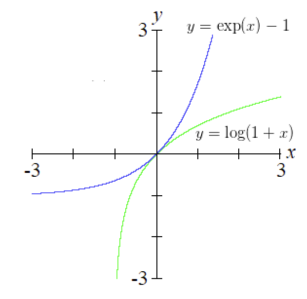
- Caveat: $y = \log(1+e^x) \to y’(x) = \frac{e^x}{1+e^x} = 1 - \sigma(-x)$
- Caveat: $y = \log(1+e^{-x}) \to y’(x) = \frac{-e^{-x}}{1+e^{-x}} = \sigma(x) - 1$
- 或是以上的 equation 是 logistic function 的積分。至於是否有用處,要再研究。
- 比較有趣的是收斂速度看起來也不錯。
$\lim_{x\to 0}\log (1 + e^{x}) \sim \lim_{x\to 0} (\log 2 +\frac{x}{2} + \frac{x^2}{8})$
$\lim_{x\to 0}\log (1 + e^{-x}) \sim \lim_{x\to 0} (\log 2 -\frac{x}{2} + \frac{x^2}{8})$
注意 $\log (1 + e^{x}) - \log (1 + e^{-x}) = x$ 這是 exact, 不是近似。
-
-
再來看 $x\to \pm \infty$
從上式:
$\lim_{x\to \infty}\log (1+e^{-x}) = \lim_{x\to \infty}(e^{-x} - \frac{e^{-2x}}{2} + …) \sim \lim_{x\to \infty} e^{-x} (\to 0^+)$
所以 $\lim_{x\to \infty}\log (1+e^{x}) = \lim_{x\to \infty}\log e^x(1+e^{-x}) \sim \lim_{x\to \infty} x + e^{-x} (\to x)$
-
什麽時候用 expm1 和 log1p?
- $x > \log 2$ 使用 log1p
- $\log (1+e^{-x}) = \text{log1p}(e^{-x})$ 或是使用近似 $e^{-x} - \frac{e^{-2x}}{2} + \frac{e^{-3x}}{3} - …$
- $\log (1+e^{x}) = \text{log1p}(e^{x}) = x + \text{log1p}(e^{-x})$ 或是使用近似 $x + e^{-x} - \frac{e^{-2x}}{2} + \frac{e^{-3x}}{3} - …$
- $x < \log 2$ 可以直接計算(因爲沒有 log 0 的問題)或是使用 expm1
- $\log (1+e^{-x}) = \log (2 + \text{expm1}(-x)) $
- $\log (1+e^{x}) = \log (2 + \text{expm1}(x)) $
- $x > \log 2$ 使用 log1p
Laplace Transform of Logistic Function
### Method 3 (2-segment)
先用簡單的例子説明:此處省略 bias, 因為 log-softmax 不會有 underflow 造成 divide by 0 問題。(不過要小心 underflow log 0 問題,不過可以用 c 解決)。所以直接看 2-dimension.
#### 2-dimension: $\mathbf{x}=\left(x_1, x_2\right) \in \text{FP16}$.
Assuming $x_1 > x_2$ Let $\widehat{x} = \max(x_1, x_2) > 0$, assuming $\widehat{x} = x_1$
\(\begin{aligned}\log\operatorname{-softmax} &=\log \left[\operatorname{softmax}(x_i)\right] \\&=\log \left(\frac{e^{x_i}}{e^{x_1}+e^{x_2}}\right) \\
&=x_i - \log \left({e^{x_1}+e^{x_2}}\right) \\
&=x_i - x_1 - \log \left({1+e^{x_2-x_1}}\right)
\end{aligned}\)
Let x = x1 - x2 > 0
$$
\begin{aligned}\log\operatorname{-softmax} &=x_i - x_1 - \log \left({1+e^{x_2-x_1}}\right)
= x_i - \widehat{x} - \log(1+e^{-x})
\end{aligned} $$ 顯然關鍵在於 log exp 項。 x 這裡是正值。可以調整到 + 11,but not help to much. 如果 $0 < x < 1$
try to use minus, then it becomes positive value! if x1 - x2 > 10 ->. Log(1+ exp(10)) ~ 10 -> 0, or x > 10, 可以忽略不計。
0< x < 1, use Taylor expansion, no underflow problem using exp()
1 < x < 5?, use another Taylor expansion, maybe still approximation ok?
Log(1+d) = d + …?
Use back-propagation for softmax? because it has a differntial equation to be correct? Use log-softmax!
分爲以下 cases:
1 | |
-
$x_1 > \beta_H > x_2$ : 直接計算 $x_1^2$ 會 overflow, 但 $x_2^2$ 不會 overflow
Let $y_1 = \frac{x_1}{\sqrt{2}}$ , $y_2 = \frac{x_2}{\sqrt{2}}$ , and $\epsilon’ = y_2^2 + \epsilon$
顯然上式沒有計算 $x_1^2$ ,不會 overflow!
比較麻煩是下面的情況:
-
$x_1, x_2 > \beta_H$ : 直接計算 $x_1^2$ 或 $x_2^2$ 都會 overflow
Let $K = \sqrt{1 + (\frac{x_2}{\widehat{x}})^2}$ where $ \sqrt{2} > K > 1$ 不會 overflow.
上式沒有計算 $x_1^2$ 或 $x_2^2$, 不會因為平方項 overflow. 因為 $K \le 1 \to $$K \widehat{x} \le \widehat{x} = \max(x_1, x_2)$ 也不會 overflow.
#### 推廣到 n-Dimension $\mathbf{x}=\left(x_1, x_2, …, x_n\right) \text{ including bias } \epsilon\in \text{FP16}$.
Let $\widehat{x} = \max(x_1, x_2, …, x_n)$
- Normal case: $\beta_H > \widehat{x}$ :直接計算 $l_2$-norm 不會 overflow. 如果 $\beta_H$ 是一個夠大 threshold, 大部分情況都是這個 case.
- Special case: $\widehat{x} > \beta_H$
-
可以分成大分量 components: $(x_1, x_2, …, x_m) > \beta_H$ 以及正常分量 components $(x_{m+1}, …, x_n) \le \beta_H $.
Let $K = \sqrt{((\frac{x_1}{\widehat{x}})^2 + … + (\frac{x_m}{\widehat{x}})^2)}$ where $\sqrt{m} \ge K \ge 1$ 不會 overflow (除非 $m \ge 65534^2, 理論上存在,實務不可能$ )
1
2
3Let $Q = x_{m+1}^2 + ... + x_n^2 + n \epsilon$ where $m < n \to S < \beta_H^2$ 不會 overflow, $Q$ 在 $n > 65534$ 有機會 overflow. 可以得到: $K^2 \widehat{x}^2 + Q = \sum_{i=1}^n x_i^2 + n \epsilon = n \|\mathbf{x}\|_2^2$ , 也就是 $l_2$-norm 的平方。因此
Taylor expansion 成立的條件: $K^2 \widehat{x}^2 > Q \to x_1^2 + \ldots +x_m^2 > x_{m+1}^2 + \ldots + x_n^2 + n \epsilon$. 物理上很有意義,就是就是大分量 vector 的 power 必須大於正常分量 vector 的 power. 這個 power ration 值愈大,Taylor expansion 近似就越準確。
定義 $\gamma = \frac{Q}{K \widehat{x}}$ , Taylor expansion 的 error term 大約是 $\gamma^2 / 8$. 如果 $\gamma < 0.3 \,\text{(30\%)}$, 相對誤差大約是 1-2%.
#### Validate $\eqref{ndimTaylor}$ using 1-dimension and 2-dimension example
1-dimension: $n = 1,\, K=(x_1/x_1)^2 = 1,\, Q = \epsilon \to |\mathbf{x}|_2 = \widehat{x} + \frac{\epsilon}{2\widehat{x}} $ Check!
2-dimension
Special case 1, $n = 2, \, K=1, \, Q=x_2^2 + 2\epsilon \to |\mathbf{x}|_2 = \frac{1}{\sqrt{2}}(\widehat{x} + \frac{x_2^2 + 2 \epsilon}{2\widehat{x}})$ Check!
Special case 2, $n = 2, \, K=\sqrt{1+(x_2/x_1)^2}, \, Q= 2\epsilon \to |\mathbf{x}|_2 = \frac{1}{\sqrt{2}}(K\widehat{x} + \frac{\epsilon}{K \widehat{x}})$ Check!
### Overflow Insight and Summary
-
首先計算 $\widehat{x} = \max(x_1, x_2, …, x_n)$: 就是 $\mathbf{x}$ 的最大 component 值。
-
再用 $\beta_H$ 作爲分界綫,如果 $\beta_H > \widehat{x}$ : 屬於 沒有 overflow 的 normal case. 直接計算 $\mathbf{x}$ 的 $l_2$-norm with bias $\epsilon$. (done)
-
如果 $\widehat{x} > \beta_H$ : 屬於 special case. Decompose $\mathbf{x} = (x_1,.., x_m, 0,..,0) + (0, ..,0, x_{m+1}, .., x_n) = \mathbf{x_K} + \mathbf{x_Q}$
where $\mathbf{x_K}$ 所有 non-zero elements 都大於 $\beta_H$ (大分量 vector), and $\mathbf{x_Q}$ 所有 non-zero elements 都小於 $\beta_H$ (正常分量 vector).
-
因此 $|\mathbf{x}|_2^2 = |\mathbf{x}|_K^2 + |\mathbf{x}|_Q^2$, 此處我們把 bias $\epsilon$ 歸在 $\mathbf{x_Q}$ 的 $l_2$ norm; $\mathbf{x_K}$ 的 bias 為 0.
-
因爲 $\mathbf{x_Q}$ 是正常分量 vector, 可以直接計算 $l_2$-norm 的平方 Q (不用開根號),不會 overflow.
-
因爲 $\mathbf{x_K}$ 是大分量 vector, 如果直接計算 $l_2$-norm, 在做平方時會 overflow, 因此需要先 normalize $\mathbf{x_K}$ with $\widehat{x}$. 再計算 normalized vector $\frac{\mathbf{x_K}}{\widehat{x}}$ 的 $l_2$-norm K. 可以避免 overflow,也就是 LAPACK 的方法。 $\mathbf{x_K}$ 的 $l_2$-norm 就是 $K \widehat{x}$ .
-
最後 $\mathbf{x} = \mathbf{x_K} + \mathbf{x_Q}$ 的 $l_2$ norm including bias 就是 $K\widehat{x}$ 加上修正項 $Q/ 2 K\widehat{x}$. (done)
-
-
1-D 和 2-D 的 case 都是 (8) 的特例。
-
(8) 只有在求 $K$ 做一次 element-wise 除法,和一個 scalar 開根號。求 $Q$ 是平方和,不需要開根號。原來的 $l_2$-norm 也需要做平方和,以及一次開根號。
-
Special case approximated $l_2$-norm 比 normal case 的 $l_2$-norm 多了 (i) 一個 (element-wise) max operation; (ii) element-wise comparison with $\beta_H$; (iii) 把原來 vector 拆成兩個 vectors; (iv) 一次 element-wise 除法; (v) 2 個 scalar 乘法,一個 scalar 除法 (除 2 right shift 省略),和一個加法。
## Underflow Problem Statement
考慮 $n$-vectors layer-norm or generalized $l_2$-norm including bias : $\mathbf{x}=\left(x_1, x_2, \ldots, x_n\right) \in \text{FP16}^n$ and a constant bias $\epsilon \in \text{FP16}$, 如何避免計算過程中 underflow 造成的精度損失。 \(\begin{aligned} \|\mathbf{x}\|_2=\sqrt{\sum_{i=1}^n x_i^2 + \epsilon} \end{aligned}\)
-
FP16 的最小值只有 $5.96\times 10^{-8}$. 如果 $\mathbf{x}$ 的 component(s) 遠小於 1 但大於最小值, i.e. $5.96\times 10^{-8}<x_i \ll 1$, 在計算 $l_2$-norm 過程中的 component(s) 的平方項很容易產生 underflow (i.e. $x_i^2<5.96\times 10^{-8}$) 影響最後 $l_2$-norm $|\mathbf{x}|_2$ 的精度。 FP32 相對沒有這個問題,因爲 FP32 的最小值為 $1.4\times 10^{-45}$.
- Extreme case: 如果有所有的 components 遠小於 1 但大於最小值, i.e. $5.96\times 10^{-8}<x_i \ll 1$, 同時 components 的平方都 underflow, i.e. $x_i^2 < 5.96\times 10^{-8}$. 最後的 $l_2$-norm 因爲 underflow 計算結果就會是 $\sqrt{\epsilon}$, 失去所有 $\mathbf{x}$ 的 information, i.e. $|\mathbf{x}|_2 = \sqrt{\epsilon}$ .
- Assumption: Underflow 發生在計算的平方項 $x_k^2$ (平方和是 sum of positive number 不會 underflow)。後的 $l_2$-norm 本身不會 underflow (i.e. $x_i^2 < 5.96\times 10^{-8}$,但是 $|\mathbf{x}|2 > 5.96\times 10^{-8}$)。此處暫時不考慮 $\epsilon \approx - \sum{i_i}^n x_i^2$ 所造成的 underflow.
- Caveat: 因爲 $x_1, x_2, …, x_n$ 是正或負,對於 (generalized) $l_2$-norm 無影響。爲了推導方便,可以假設 $x_1, …, x_n \ge 0$. 如果 $x_i < 0$, 就改成 $-x_i > 0$ 不影響 $l_2$-norm 的計算。 Bias $\epsilon$ 可正可負。
###
第 2 节中我们按照数学定义分别定义了 softmax 函数和 CrossEntropy 损失,这样做可能导致数据不稳定
softmax 函数定义为 y ^ i = exp ( o i ) ∑ j exp ( o j ) \hat{y}_i = \frac{\exp(o_i)}{\sum_j \exp(o_j)} y
i
= ∑ j
exp(o j
) exp(o i
)
注意这里都是 exp 运算,一旦网络初始化不当,或输入数值有较大噪音,很可能导致数值溢出(o oo 是很大的正整数会导致上溢,o oo 是很大的负整数会导致下溢),这时可以用 Log-Sum-Exp Trick(logSoftmax)处理,它在数学上就是在普通 softmax 外面套了一个 log 函数,这不会影响概率排序,但是通过有技巧地实现可以有效解决溢出问题。具体参考 深入理解softmax CrossEntropy损失在这里为 H ( y ( i ) , y ^ ( i ) ) = − ∑ j = 1 q y j ( i ) log y ^ j ( i ) = − log y ^ y ( i ) ( i ) H(\pmb{y}^{(i)},\hat{\pmb{y}}^{(i)}) = -\sum_{j=1}^q y_j^{(i)}\log\hat{y}j^{(i)} = -\log\hat{y}{y^{(i)}}^{(i)} H( y y (i) , y y ^
(i) )=− j=1 ∑ q
y j (i)
log y ^
j (i)
=−log y ^
y (i)
(i)
当 y ^ y ( i ) ( i ) \hat{y}_{y^{(i)}}^{(i)} y ^
y (i)
(i)
1 | |
i=1 ∑ n
−log y ^
y (i)
(i)
如果已经用 logSoftmax计算了各个 log y ^ y ( i ) ( i ) \log\hat{y}_{y^{(i)}}^{(i)}log y ^
y (i)
(i)
,可以直接用负对数似然方法 torch.NLLLoss 方法得到 l ( Θ ) \mathscr{l}(\Theta)l(Θ)。NLLLosss 的具体行为可以参考 loss函数之NLLLoss,CrossEntropyLoss 总之,我们可以用 logSoftmax + NLLLoss 避免数据溢出,保证数据稳定性,并且得到等价的交叉熵损失,pytorch 中直接把这两个放在一起封装了一个 nn.CrossEntropyLoss 方法,对于一组小批量数据,假设模型输出和真实标签分别为 o u t p u t outputoutput 和 t r u t h truthtruth, nn.CrossEntropyLoss 如下计算小批量损失 ———————————————— 版权声明:本文为CSDN博主「云端FFF」的原创文章,遵循CC 4.0 BY-SA版权协议,转载请附上原文出处链接及本声明。 原文链接:https://blog.csdn.net/wxc971231/article/details/124629256
### Method 1 (with underflow side-effect)
Public Linear Algebra PACKage LAPACK 的做法是 normalized to maximum $x_i$
Let Let $\widehat{x} = \max(x_1, x_2, …, x_n)$ \(\begin{align} \|\mathbf{x}\|_2 = \frac{\widehat{x}}{\sqrt{n}} \times\|\mathbf{x} / \widehat{x}\|_2 \end{align}\) where $\widehat{x}=\max(x_1, x_2, …, x_n)$.
-
這個方法把 normalized $l_2$-norm, $|\mathbf{x} / \widehat{x}|_2$ , 所有的 components 都控制小於等於 1, 避免 overflow. 對於 FP32 沒有問題 ( FP32 的範圍 [$1.4\times 10^{-45}, 3.4\times 10^{38}$] )。
-
但對於 FP16 可能會有 underflow (i.e. $x_k^2 < 5.96\times 10^{-8}$) 造成精度損失的問題。
-
Extreme case: 如果有一個 component 遠大於其他所有 components, i.e. $x_k = \widehat{x} \gg x_i$, 最後的 $l_2$-norm 因爲 underflow 計算結果就會是 $\widehat{x}$, 失去所有其他 component 的 information, i.e. $|\mathbf{x}|_2 = \widehat{x} \times|\mathbf{x} / \widehat{x}|_2 / \sqrt{n} = \widehat{x}/\sqrt{n}$ .
### Method 2 (2-segment)
先用簡單的例子説明:
#### 1-dimension: $\mathbf{x}=\left(x_1\right) \text{ including bias } \epsilon\in \text{FP16}$
\[\begin{align*} \|\mathbf{x}\|_2 &=\sqrt{x_1^2 + \epsilon} \end{align*}\]我們可以用 $\beta_H > 0$ 把定義域分成兩段: $x_1 \ge \beta_H$ or $x_1 < \beta_H$. 假設 $\epsilon < \beta_H^2 $.
-
Normal case: $x_1 \le \beta_H$ , 直接計算 $l_2$-norm. 如果 $\beta_H$ 是一個大的 threshold, 大多數情況都是這個 case. For example, $\beta_H = \sqrt{65504} \approx 256$.
-
Special case: $x_1 > \beta_H$, 如果直接計算 $l_2$-norm,在計算 $x_1^2$ 就會 overflow.
此時可以利用 Taylor expansion 避免計算平方項: $\sqrt{1+x} = 1+\frac{x}{2}-\frac{x^2}{8}+\frac{x^3}{16}-\frac{5 x^4}{128}+\frac{7 x^5}{256}+ … = 1+\frac{x}{2}+O(x^2)$
- 選擇 $\beta_H$ 對於 $\epsilon$ ratio 要夠大,才能確保 relative error 夠小。
#### 2-dimension: $\mathbf{x}=\left(x_1, x_2\right) \text{ including bias } \epsilon\in \text{FP16}$.
\[\begin{aligned}\|\mathbf{x}\|_2 &=\sqrt{\frac{x_1^2 + x_2^2}{2} + \epsilon}\end{aligned}\]Let $\widehat{x} = \max(x_1, x_2) > 0$, assuming $\widehat{x} = x_1$
分爲以下 cases:
- Normal case: $\beta_H > \widehat{x}$ :直接計算 $l_2$-norm 不會 overflow. 如果 $\beta_H$ 是一個夠大 threshold, 大部分情況都是這個 case.
- Special case: $\widehat{x} (= x_1) > \beta_H$, 分爲兩種情況
-
$x_1 > \beta_H > x_2$ : 直接計算 $x_1^2$ 會 overflow, 但 $x_2^2$ 不會 overflow
Let $y_1 = \frac{x_1}{\sqrt{2}}$ , $y_2 = \frac{x_2}{\sqrt{2}}$ , and $\epsilon’ = y_2^2 + \epsilon$
顯然上式沒有計算 $x_1^2$ ,不會 overflow!
比較麻煩是下面的情況:
-
$x_1, x_2 > \beta_H$ : 直接計算 $x_1^2$ 或 $x_2^2$ 都會 overflow
Let $K = \sqrt{1 + (\frac{x_2}{\widehat{x}})^2}$ where $ \sqrt{2} > K > 1$ 不會 overflow.
上式沒有計算 $x_1^2$ 或 $x_2^2$, 不會因為平方項 overflow. 因為 $K \le 1 \to $$K \widehat{x} \le \widehat{x} = \max(x_1, x_2)$ 也不會 overflow.
#### 推廣到 n-Dimension $\mathbf{x}=\left(x_1, x_2, …, x_n\right) \text{ including bias } \epsilon\in \text{FP16}$.
Let $\widehat{x} = \max(x_1, x_2, …, x_n)$
- Normal case: $\beta_H > \widehat{x}$ :直接計算 $l_2$-norm 不會 overflow. 如果 $\beta_H$ 是一個夠大 threshold, 大部分情況都是這個 case.
- Special case: $\widehat{x} > \beta_H$
-
可以分成大分量 components: $(x_1, x_2, …, x_m) > \beta_H$ 以及正常分量 components $(x_{m+1}, …, x_n) \le \beta_H $.
Let $K = \sqrt{((\frac{x_1}{\widehat{x}})^2 + … + (\frac{x_m}{\widehat{x}})^2)}$ where $\sqrt{m} \ge K \ge 1$ 不會 overflow (除非 $m \ge 65534^2, 理論上存在,實務不可能$ )
1
2
3
Let $Q = x_{m+1}^2 + ... + x_n^2 + n \epsilon$ where $m < n \to S < \beta_H^2$ 不會 overflow, $Q$ 在 $n > 65534$ 有機會 overflow. 可以得到: $K^2 \widehat{x}^2 + Q = \sum_{i=1}^n x_i^2 + n \epsilon = n \|\mathbf{x}\|_2^2$ , 也就是 $l_2$-norm 的平方。因此 $$ \begin{align} \|\mathbf{x}\|_2 &= \sqrt{(x_1^2 + x_2^2 + ... + x_m^2 + x_{m+1}^2 + ...x_n^2)/n + \epsilon} \nonumber\ &= \sqrt{\frac{K^2 \widehat{x}^2 + Q}{n} } \nonumber\ &= \frac{K \widehat{x}}{\sqrt{n}} \sqrt{1 + \frac{Q}{K^2 \widehat{x}^2}} \nonumber\ &\approx \frac{K \widehat{x}}{\sqrt{n}} (1 + \frac{Q }{2 K^2 \widehat{x}^2}) \nonumber\ &= \frac{1}{\sqrt{n}}(K \widehat{x} + \frac{Q}{2K\widehat{x}}) \label{ndimTaylor} \end{align} $$
Taylor expansion 成立的條件: $K^2 \widehat{x}^2 > Q \to x_1^2 + \ldots +x_m^2 > x_{m+1}^2 + \ldots + x_n^2 + n \epsilon$. 物理上很有意義,就是就是大分量 vector 的 power 必須大於正常分量 vector 的 power. 這個 power ration 值愈大,Taylor expansion 近似就越準確。
定義 $\gamma = \frac{Q}{K \widehat{x}}$ , Taylor expansion 的 error term 大約是 $\gamma^2 / 8$. 如果 $\gamma < 0.3 \,\text{(30\%)}$, 相對誤差大約是 1-2%.
#### Validate $\eqref{ndimTaylor}$ using 1-dimension and 2-dimension example
1-dimension: $n = 1,\, K=(x_1/x_1)^2 = 1,\, Q = \epsilon \to |\mathbf{x}|_2 = \widehat{x} + \frac{\epsilon}{2\widehat{x}} $ Check!
2-dimension
Special case 1, $n = 2, \, K=1, \, Q=x_2^2 + 2\epsilon \to |\mathbf{x}|_2 = \frac{1}{\sqrt{2}}(\widehat{x} + \frac{x_2^2 + 2 \epsilon}{2\widehat{x}})$ Check!
Special case 2, $n = 2, \, K=\sqrt{1+(x_2/x_1)^2}, \, Q= 2\epsilon \to |\mathbf{x}|_2 = \frac{1}{\sqrt{2}}(K\widehat{x} + \frac{\epsilon}{K \widehat{x}})$ Check!
### Overflow Insight and Summary
-
首先計算 $\widehat{x} = \max(x_1, x_2, …, x_n)$: 就是 $\mathbf{x}$ 的最大 component 值。
-
再用 $\beta_H$ 作爲分界綫,如果 $\beta_H > \widehat{x}$ : 屬於 沒有 overflow 的 normal case. 直接計算 $\mathbf{x}$ 的 $l_2$-norm with bias $\epsilon$. (done)
-
如果 $\widehat{x} > \beta_H$ : 屬於 special case. Decompose $\mathbf{x} = (x_1,.., x_m, 0,..,0) + (0, ..,0, x_{m+1}, .., x_n) = \mathbf{x_K} + \mathbf{x_Q}$
where $\mathbf{x_K}$ 所有 non-zero elements 都大於 $\beta_H$ (大分量 vector), and $\mathbf{x_Q}$ 所有 non-zero elements 都小於 $\beta_H$ (正常分量 vector).
-
因此 $|\mathbf{x}|_2^2 = |\mathbf{x}|_K^2 + |\mathbf{x}|_Q^2$, 此處我們把 bias $\epsilon$ 歸在 $\mathbf{x_Q}$ 的 $l_2$ norm; $\mathbf{x_K}$ 的 bias 為 0.
-
因爲 $\mathbf{x_Q}$ 是正常分量 vector, 可以直接計算 $l_2$-norm 的平方 Q (不用開根號),不會 overflow.
-
因爲 $\mathbf{x_K}$ 是大分量 vector, 如果直接計算 $l_2$-norm, 在做平方時會 overflow, 因此需要先 normalize $\mathbf{x_K}$ with $\widehat{x}$. 再計算 normalized vector $\frac{\mathbf{x_K}}{\widehat{x}}$ 的 $l_2$-norm K. 可以避免 overflow,也就是 LAPACK 的方法。 $\mathbf{x_K}$ 的 $l_2$-norm 就是 $K \widehat{x}$ .
-
最後 $\mathbf{x} = \mathbf{x_K} + \mathbf{x_Q}$ 的 $l_2$ norm including bias 就是 $K\widehat{x}$ 加上修正項 $Q/ 2 K\widehat{x}$. (done)
-
-
1-D 和 2-D 的 case 都是 (8) 的特例。
-
(8) 只有在求 $K$ 做一次 element-wise 除法,和一個 scalar 開根號。求 $Q$ 是平方和,不需要開根號。原來的 $l_2$-norm 也需要做平方和,以及一次開根號。
-
Special case approximated $l_2$-norm 比 normal case 的 $l_2$-norm 多了 (i) 一個 (element-wise) max operation; (ii) element-wise comparison with $\beta_H$; (iii) 把原來 vector 拆成兩個 vectors; (iv) 一次 element-wise 除法; (v) 2 個 scalar 乘法,一個 scalar 除法 (除 2 right shift 省略),和一個加法。
## Underflow Problem Statement
考慮 $n$-vectors layer-norm or generalized $l_2$-norm including bias : $\mathbf{x}=\left(x_1, x_2, \ldots, x_n\right) \in \text{FP16}^n$ and a constant bias $\epsilon \in \text{FP16}$, 如何避免計算過程中 underflow 造成的精度損失。 \(\begin{aligned} \|\mathbf{x}\|_2=\sqrt{\sum_{i=1}^n x_i^2 + \epsilon} \end{aligned}\)
-
FP16 的最小值只有 $5.96\times 10^{-8}$. 如果 $\mathbf{x}$ 的 component(s) 遠小於 1 但大於最小值, i.e. $5.96\times 10^{-8}<x_i \ll 1$, 在計算 $l_2$-norm 過程中的 component(s) 的平方項很容易產生 underflow (i.e. $x_i^2<5.96\times 10^{-8}$) 影響最後 $l_2$-norm $|\mathbf{x}|_2$ 的精度。 FP32 相對沒有這個問題,因爲 FP32 的最小值為 $1.4\times 10^{-45}$.
- Extreme case: 如果有所有的 components 遠小於 1 但大於最小值, i.e. $5.96\times 10^{-8}<x_i \ll 1$, 同時 components 的平方都 underflow, i.e. $x_i^2 < 5.96\times 10^{-8}$. 最後的 $l_2$-norm 因爲 underflow 計算結果就會是 $\sqrt{\epsilon}$, 失去所有 $\mathbf{x}$ 的 information, i.e. $|\mathbf{x}|_2 = \sqrt{\epsilon}$ .
- Assumption: Underflow 發生在計算的平方項 $x_k^2$ (平方和是 sum of positive number 不會 underflow)。後的 $l_2$-norm 本身不會 underflow (i.e. $x_i^2 < 5.96\times 10^{-8}$,但是 $|\mathbf{x}|2 > 5.96\times 10^{-8}$)。此處暫時不考慮 $\epsilon \approx - \sum{i_i}^n x_i^2$ 所造成的 underflow.
- Caveat: 因爲 $x_1, x_2, …, x_n$ 是正或負,對於 (generalized) $l_2$-norm 無影響。爲了推導方便,可以假設 $x_1, …, x_n \ge 0$. 如果 $x_i < 0$, 就改成 $-x_i > 0$ 不影響 $l_2$-norm 的計算。 Bias $\epsilon$ 可正可負。
### Method 1 (help in some case, mostly worse)
Public Linear Algebra PACKage LAPACK 的做法是 normalized to maximum $x_i$.
Let $\widehat{x} = \max(x_1, x_2, …, x_n)$ \(\|\mathbf{x}\|_2 = \widehat{x} \times\|\mathbf{x} / \widehat{x}\|_2\) where $\widehat{x}=\max(x_1, x_2, …, x_n)$.
- normalized $l_2$-norm, $|\mathbf{x} / \widehat{x}|_2$ , 所有的 components 都控制小於等於 1. 對於 FP32 沒有問題 ( FP32 的範圍 [$1.4\times 10^{-45}, 3.4\times 10^{38}$] )。
- 對於 FP16 這個方法只有在所有的 components $x_i$ 都遠小於 1 才有幫助, i.e. $5.96\times 10^{-8}<x_i, \epsilon \ll 1$. 因爲 $\widehat{x}=\max(x_1, …, x_n) < 1$, normalized vector $|\mathbf{x} / \widehat{x}|_2$ 會把所有的 components 放大。不過最大的component 也只放大到 1,只能減輕 underflow.
- (remove) Bias 需要小於 1, i.e. $\epsilon<1$, 不然 bias 放大反而容易造成 overflow, i.e. $\epsilon / \widehat{x} > 65504$.
- 最大的問題是任何一個 $x_i > 1 \to \widehat{x} > 1$, normalized vector $|\mathbf{x} / \widehat{x}|_2$ 會把所有的 components 縮小。只會讓 underflow 問題更 worse.
- 結論: Method 1 在大部分的情況 (any $x_i > 1$),只會讓 underflow 問題更 worse.
### Method 2 (2-segment)
先用簡單的例子説明:
#### 1-dimension: $\mathbf{x}=\left(x_1\right) \text{ including bias } \epsilon\in \text{FP16}$
\[\begin{aligned} \|\mathbf{x}\|_2 &=\sqrt{x_1^2 + \epsilon} \end{aligned}\]我們可以用 $1 > \beta_L$ 把定義域分成兩段: $x_1 \ge \beta_L$ or $x_1 < \beta_L$.
-
Normal case: $x_1 \ge \beta_L$ , 直接計算 $l_2$-norm. 如果 $\beta_L$ 是一個遠小於 1 的 threshold 但大於等於 FP16 最小精度的平方根,可以避免計算平方時 underflow, i.e. $1 \gg \beta_L > \sqrt{FP16_{min}}$. 大部分情況都是這個 case. 例如我們可以取 $\beta_L = \sqrt{5.96\times 10^{-8}} = 2.4\times 10^{-4}$.
-
Special case: $x_1 < \beta_L \,(2.4\times 10^{-4})$ , 如果直接計算 $l_2$-norm,在計算 $x_1^2$ 就會 underflow. 我們先把上式變形:
到目前爲止都是 exact, 沒有任何近似。對於 non-zero ** $\epsilon \in \text{FP16} \to \sqrt{\epsilon} \in \text{FP16}$ **不會有 underflow. 主要的問題是 $x_1^2 < \beta_L^2$ 會 underflow.
接下來計算判別式:
\(\gamma = \frac{x_1}{\sqrt{\epsilon}}\)
-
如果 $\gamma \ge \beta_L = 2.4\times 10^{-4}$ : 代表 $\epsilon < 1$, $x_i (<\beta_L)$ 除以 $\sqrt{\epsilon}$ 可以放大 $x_1$ 避免 underflow. 可以直接用 (12) 計算 $l_2$-norm 如下: \(\begin{aligned}\|\mathbf{x}\|_2 &=\sqrt{x_1^2 + \epsilon} \\ &= \sqrt{\epsilon} \sqrt{1+ \left(\frac{x_1}{\sqrt{\epsilon}}\right)^2}\\ &= \sqrt{\epsilon} \sqrt{1+ \gamma^2} \end{aligned}\)
-
如果 $\gamma < \beta_L = 2.4\times 10^{-4}$ : 利用 Taylor expansion
\(\begin{aligned}\|\mathbf{x}\|_2 &=\sqrt{x_1^2 + \epsilon} \\ &= \sqrt{\epsilon} \sqrt{1+ \left(\frac{x_1}{\sqrt{\epsilon}}\right)^2}\\ &= \sqrt{\epsilon} \sqrt{1+ \gamma^2} \\ & \approx \sqrt{\epsilon} (1+ \frac{\gamma^2}{2}) = \sqrt{\epsilon} + \frac{(\sqrt{\epsilon}\gamma)\gamma}{2} \end{aligned}\) 除非 $\epsilon > 1$, $\sqrt{\epsilon} \gamma $ 可以把 $\gamma$ 放大到 underflow threshold 以上,不然第二 (修正) 項在 FP16 dynamic range 無法 cover.
#### n-Dimension $\mathbf{x}=\left(x_1, x_2, …, x_n\right) \text{ including bias } \epsilon\in \text{FP16}$.
Let $x_{min} = \min(x_1, x_2, …, x_n)$
我們可以用 $1 > \beta_L > 0$ 把定義域分成兩段: $x_1 \ge \beta_L$ or $x_1 < \beta_L$.
- Normal case: $x_{min} \ge \beta_L$ , 直接計算 $l_2$-norm. 如果 $\beta_L$ 是一個遠小於 1 的 threshold $1 \gg \beta_L$, 大部分情況都是這個 case. For example, $\beta_L = \sqrt{5.96\times 10^{-8}} = 2.4\times 10^{-4}$.
- Special case: $x_{min} < \beta_L$
-
可以分成小分量 components: $(x_1, x_2, …, x_m) < \beta_L$ 以及正常分量 components $(x_{m+1}, …, x_n) \ge \beta_L $.
Let $K^2 = (\frac{x_1}{\tilde{x}})^2 + … + (\frac{x_m}{\tilde{x}})^2$ where $\tilde{x} = \max(x_1, .., x_m)$
Let $Q^2 = x_{m+1}^2 + … + x_n^2 + \epsilon$
-
Caveat 1: $\tilde{x} < \beta_L = 2.4\times 10^{-4}$ and $\sqrt{m} > K > 1$
-
Caveat 2: $Q > (n-m+1) \beta_L + \epsilon $
可以得到: $K^2 \tilde{x}^2 + Q^2 = \sum_{i=1}^n x_i^2 + \epsilon = |\mathbf{x}|_2^2$ , 也就是 $l_2$-norm 的平方。因此
到目前爲止都是 exact, 沒有任何近似。$K>1$ 不會有 underflow 問題。$Q$ 是正常分量的 $l_2$-norm, 也沒有 underflow 的問題。唯一的問題是 $\tilde{x}^2 < \beta_L^2 = 5.96\times 10^{-8}$ 會有 underflow 的問題。
接下來計算判別式:
\(\gamma = \frac{K\tilde{x}}{Q}\)
-
如果 $\gamma > \beta_L = 2.4\times 10^{-4}$, 直接利用 (16) 計算 $|\mathbf{x}|_2 $ 如下式。不會有 underflow 問題, done. \(\begin{aligned}\|\mathbf{x}\|_2 &=\sqrt{x_1^2 + x_2^2 + ... + x_m^2 + x_{m+1}^2 + ...x_n^2 + \epsilon} \\&= \sqrt{K^2 \tilde{x}^2 + Q^2} \\&= Q \sqrt{1 + \frac{K^2\tilde{x}^2}{Q^2}} \\ &= Q \sqrt{1+\gamma^2} \end{aligned}\)
-
如果 $\gamma \le \beta_L = 2.4\times 10^{-4}$, 利用 Taylor expansion again:
如果 $Q > 1$, 就是利用 $Q$ 把 $\gamma$ 放大,避免 underflow 的問題。如果 $Q < 1$, 代表小分量無法用 FP16 精度表示, done.
### Underflow Insight and Summary
-
首先計算 $x_{min} = \min(x_1, x_2, …, x_n)$: 就是 $\mathbf{x}$ 的最小 component 值。
-
再用 $\beta_L$ 作爲分界綫,如果 $x_{min} \ge \beta_L$ : 屬於沒有 underflow 的 normal case. 直接計算 $\mathbf{x}$ 的 $l_2$-norm with bias $\epsilon$. (done)
-
如果 $x_{min} < \beta_L$ : 屬於 special case. Decompose $\mathbf{x} = (x_1,.., x_m, 0,..,0) + (0, ..,0, x_{m+1}, .., x_n) = \mathbf{x_K} + \mathbf{x_Q}$
where $\mathbf{x_K}$ 所有 non-zero elements 都小於 $\beta_L$ (小分量 vector), and $\mathbf{x_Q}$ 所有 non-zero elements 都大於 $\beta_H$ (正常分量 vector). 此時要多做一個 $\mathbf{x_K}$ 的 max: $\tilde{x} = \max(x_1, .., x_m, 0, ..0)$
- 因此 $|\mathbf{x}|_2^2 = |\mathbf{x}|_K^2 + |\mathbf{x}|_Q^2$, 此處我們把 bias $\epsilon$ 歸在 $\mathbf{x_Q}$ 的 $l_2$ norm; $\mathbf{x_K}$ 的 bias 為 0.
- 因爲 $\mathbf{x_Q}$ 是正常分量 vector, 可以直接計算 $l_2$-norm Q,不會 underflow.
- 因爲 $\mathbf{x_K}$ 是小分量 vector, 如果直接計算 $l_2$-norm, 在做平方時會 underflow, 因此需要先 normalize $\mathbf{x_K}$ with $\tilde{x}$. 再計算 normalized vector $\frac{\mathbf{x_K}}{\tilde{x}}$ 的 $l_2$-norm K, 可以避免 underflow. $\mathbf{x_K}$ 的 $l_2$-norm 就是 $K \tilde{x}$ .
- 計算判別式 $\gamma = \frac{K\tilde{x}}{Q}$ , 如果 $\gamma > \beta_L$, $|\mathbf{x}|_2 = Q \sqrt{1+\gamma^2}$ 沒有 underflow (done)
- 如果 $\gamma < \beta_L$, 利用 Taylor expansion: $|\mathbf{x}|_2 = Q + (Q\gamma)\gamma/2$ (done)
-
Special case $l_2$-norm 比 normal case 的 $l_2$-norm 多了 (i) 一個 (element-wise) min 和一個max operation; (ii) element-wise comparison with $\beta_L$; (iii) 把原來 vector 拆成兩個 vectors; (iv) 一次 element-wise 除法; (v) 還有幾個 scalar 乘法,除法,和開根號。
推廣到 n-Dimension $\mathbf{x}=\left(x_1, x_2, …, x_n\right) \text{ including bias } \epsilon\in \text{FP16}$.
Let $\widehat{x} = \max(x_1, x_2, …, x_n)$
- Normal case: $\beta_H > \widehat{x}$ :直接計算 $l_2$-norm 不會 overflow. 如果 $\beta_H$ 是一個夠大 threshold, 大部分情況都是這個 case.
- Special case: $\widehat{x} > \beta_H$
-
可以分成大分量 components: $(x_1, x_2, …, x_m) > \beta_H$ 以及正常分量 components $(x_{m+1}, …, x_n) \le \beta_H $.
Let $K = \sqrt{((\frac{x_1}{\widehat{x}})^2 + … + (\frac{x_m}{\widehat{x}})^2)/m}$ where $K \le 1$ 不會 overflow
1
2
3
Let $n Q^2 = x_{m+1}^2 + ... + x_n^2 + n \epsilon$ ($m < n$, 一般 $m \ll n$) where $Q < \beta_H$ 不會 overflow 可以得到: $K^2 m \widehat{x}^2 + Q^2 = \sum_{i=1}^n x_i^2 + n \epsilon = n \|\mathbf{x}\|_2^2$ , 也就是 $l_2$-norm 的平方。因此 $$ \begin{aligned}\|\mathbf{x}\|_2 &= \sqrt{(x_1^2 + x_2^2 + ... + x_m^2 + x_{m+1}^2 + ...x_n^2)/n + \epsilon} \ &= \sqrt{\frac{m K^2 \widehat{x}^2 + n Q^2}{n} } \ &= K \widehat{x} \sqrt{1 + \frac{n Q^2}{m K^2 \widehat{x}^2}} \sqrt{\frac{m}{n}}\ &\approx K \widehat{x} (1 + \frac{n Q^2 }{2 m K^2 \widehat{x}^2})\sqrt{\frac{m}{n}}\ &= K \widehat{x} \sqrt{\frac{m}{n}} + \frac{Q^2}{2K\widehat{x}}\sqrt{\frac{n}{m}} \end{aligned} $$
where $Q^2 < \beta_H^2, m K^2 \widehat{x}^2 > m \beta_H^2$, 所以 Taylor series 會收斂。
Check special case 1-D: m = 1, n = 1 : $Q^2 = \epsilon$ and $K=(x_1/x_1)^2 = 1 \to |\mathbf{x}|_2 = \widehat{x} + \frac{\epsilon}{2\widehat{x}} $ Yes!
Check special case 2-D (a): m = 1, n = 2 : $K^2 = (x_1/x_1)^2 = 1 \to K = 1$
$2 Q^2 = x_2^2 + 2 \epsilon \to Q^2 = x_2^2/2 + \epsilon$
$|\mathbf{x}|_2 = \frac{\widehat{x}}{\sqrt{2}} + \sqrt{2}\frac{x_2^2/2+\epsilon}{2 \widehat{x}} = \frac{1}{\sqrt{2}}(\widehat{x}+\frac{x_2^2 + 2\epsilon}{2\widehat{x}}) $ Yes!
Check special case 2-D (b): m = 2, n = 2 : $2 K^2 = (x_1/x_1)^2 + (x_2/x_1)^2 = 1 + (x_2/x_1)^2 $, and $Q^2 = \epsilon$
$|\mathbf{x}|_2 = K {\widehat{x}} + \frac{\epsilon}{2 K \widehat{x}}$ Yes!
Is is better to choose? : $\sqrt{n} Q’^2 = x_{m+1}^2 + … + x_n^2 + n \epsilon \to \sqrt{n} Q’^2 = n Q^2 \to \sqrt{n} Q^2 = Q’^2$
therefore: \(\begin{aligned}\|\mathbf{x}\|_2 &\approx K \widehat{x} \sqrt{\frac{m}{n}} + \frac{Q^2}{2K\widehat{x}}\sqrt{\frac{n}{m}} \\ &= K \widehat{x} \sqrt{\frac{m}{n}} + \frac{Q'^2}{2K\widehat{x}\sqrt{m}} \end{aligned}\)
####
Further task:
-
Reduce computation complexity
-
multiply by power of 2, divide by power of 2, the constant can be arbitrary value
-
catch: Kx_bar, 所以可以是 2^power, no need to be max. => task!
-
-
Other format:
- FP8, BF16, DLF16, etc.
- DFL16, FP8 different format, beta and scaling factor
- parameter choose is very interesting!
-
Improve the flexibility (for FP8, …)
- Assuming sign-bit can be used because of norm is positive (change neg to pos)
-
How about scaler multiplication use FP32? to solve the problem once for all!
- 如果讓 scalar (not vector) engine support FP32, 是否有好處?
Appendix
Appendix A: $\log(1+e^x)$
\(\begin{aligned} &\text{Let } \mathrm{y}=\log \left(1+\mathrm{e}^{\mathrm{x}}\right) \\ &\mathrm{y}(0)=\log 2 \\ &\text {Now } \quad y_1=\frac{e^x}{1+e^x} \\ &y_1(0)=\frac{1}{2} \\ &y_2=\frac{e^x}{\left(1+e^x\right)^2}=\frac{e^x}{1+e^x} \cdot \frac{1}{1+e^x}=y_1\left(1-y_1\right) \\ &y_2(0)=\frac{1}{2}\left(1-\frac{1}{2}\right)=\frac{1}{4} \\ &\therefore y_3=y_1\left(-y_2\right)+\left(1-y_1\right) y_2=y_2-2 y_1 y_2 \\ &\therefore \quad y_3(0)=\frac{1}{4}-2 \cdot \frac{1}{2} \cdot \frac{1}{4}=0 \\ &y_4=y_3-2\left(y_1 y_3+y_2^2\right) \\ &y_4(0)=0-2\left(\frac{1}{2} \cdot 0+\frac{1}{16}\right)=\frac{-1}{8} \end{aligned}\) Therefore from Maclaurin’s theorem, we get \(\begin{aligned} &y=y(0)+x y_1(0)+\frac{x^2}{2 !} y_2(0)+\ldots \ldots . \\ &\log \left(1+e^4\right)=\log 2+x \cdot \frac{1}{2}+\frac{x^2}{2 !} \cdot \frac{1}{4} \\ &\quad+\frac{x^3}{3 !}(0)+\frac{x^4}{4 !}\left(-\frac{1}{8}\right)+\ldots \ldots . . \\ &\log \left(1+e^4\right)=\log 2 \\ &\quad+\frac{x}{2}+\frac{x^2}{8}-\frac{x^4}{192}+\ldots \ldots . \end{aligned}\)