Reference
Cohere 在 natural language processing 出了幾篇介紹的文章都非常有幫助。
[@serranoWhatAre2023] : excellent introduction of embedding
[@serranoWhatSemantic2023] : excellent introduction of semantic search
https://txt.cohere.ai/what-is-semantic-search/
@alammarIllustratedGPT2Visualizing2022
@wolfeGivenIncredible2023
Introduction
NLP 最有影響力的幾個觀念包含 embedding, attention (query, key, value). 之後也被其他領域使用。例如 computer vision, ….
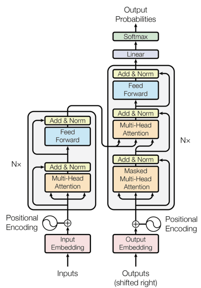
Embedding 並非 transformer 開始。最早是 starting from word2vec paper.
QKV: query, key, value 這似乎最早是從 database 或是 recommendation system 而來。從 transformer paper 開始聲名大噪,廣汎用於 NLP, vision, voice, etc.
attention: 特別是 self-attention, 然後才是 cross-attention. 雖然在 RNN 已經有 attention 的觀念,但是到 transformer 才發揚光大。 RNN 其實已經有時序的 attention, 在加上 attention 似乎有點畫蛇添足。Transformer attention 是 spatial attention, 並且範圍更大。
QKV 直觀意義和對應的數學:
直觀意義在前,對應的數學在冒號後。
- (Learnable) Input Embedding: 把 input token (words or sub-words) 一一轉換成 fixed dimension embedding/vector
- (Not learnable) Embedding similarity: 計算每個 Q embedding 對所有其他 K embeddings 的相似性,使用 vector-vector 的點積
- (Not learnable) 計算 weighed sum of V embeddings. Weights 稱爲 attention = softmax(QK^T/sqrt(d_k)) V
- (Learnable) Mutli-head attention
- (Learnable) Feed-forward
Vector Based QKV
-
(Character, Word, Sentence level, C/W/S) Embedding attention: scaled dot-product similarity,
-
Attention weight: softmax
-
(C/W/S) Embedding similarity: Weighed sum of attention
-
Multi-level (C/W/S) and multiple (word ambiguity) embeddings similarity: Mutli-head attention learning
QKV 其他的數學模式?
Manifold
前面的 vector QKV 可以視爲歐式空間。Manifold 可以想象就是非歐 (曲率) 空間。另一種類似的手法就是 kernel space.
對我而言,
- Manifold 是 local 近似歐式空間,但是 global 是曲率空間
- Kernel 是 local 曲率空間,global 類似歐式空間
- 當然兩者可以合在一起變成 local and global 都是曲率空間
然而歐式空間的計算非常友好,例如 matrix, dot-product 都有快速平行的運算。只有高維度的 softmax 計算比較麻煩一點。
曲率空間連算個距離都非常複雜。除非有特別的好處。不然把計算推到曲率空間只是自找麻煩。
假如曲率空間可以用比較低維度的計算,也許值得探索。
不過老實說,目前我看到的曲率空間用於 machine learning, 多半是理論階段。例如 information geometry. 數學, notation 上很精簡漂亮,但是離實用有一大段的距離。光看愛因斯坦的廣義相對論就知道,即使簡單的 boundary condition 的 manifold 都非常複雜。
Graph
Graph 從一個角度可以視爲更原始的幾何或是拓撲。乾脆用 connection 取代 metric. 當然我們還是可以在 connection 加上距離提供一些 metric information. 不過 graph 一般是非常 nonlinear.
如果 manifold 都有困難,使用 graph 豈不是更難? 而且好處在哪裏?
可能的好處
- text or language 的 embedding 好像用 graphic 描述更自然?或是更 compact?
- graphic 的數學可能完全不同,例如 random traverse, diffusion. 從 graph 也許更有物理意義?
這套 matrix 乘法 -> softmax -> linear combination .. 是否有類似的應用和數學 frame work?
應用: information retrieval, database management, recommendation system
數學 frame work: Graph?
- Embedding 不是向量,而是 nodes of graphs?
- Attention/Similarity 是用 neighborhood connection (or diffusion distance)
- Multi-level similarity : clustering?
Semantic Search for QKV
在我們學習語義搜索 (semantic search) 之前,讓我們看看什麼不是語義搜索。在語義搜索之前,最流行的搜索方式是關鍵字搜索 (keyword search)。想像一下,你有一個包含許多句子的清單,這些句子是回應。當您提出問題(查詢)時,關鍵字搜索會查找與查詢共有的單詞數最多的句子(回應)。例如,請考慮以下查詢和一組回應:
Query: Where is the world cup?
Responses:
-
The world cup is in Qatar.
-
The sky is blue.
-
The bear lives in the woods.
-
An apple is a fruit.
使用關鍵字搜索,您會注意到響應與查詢有以下相同的單詞數:
Responses:
- The world cup is in Qatar. (4 words in common)
- The sky is blue. (2 words in common)
- The bear lives in the woods. (2 words in common)
- An apple is a fruit. (1 word in common)
In this case, the winning response is number 1, “The world cup is in Qatar”. This is the correct response, luckily. However, this won’t always be the case. Imagine if there was another response:
- Where in the world is my cup of coffee?
這個響應與查詢有 5 個相同的詞,所以如果它在響應列表中,它就會獲勝。這很不幸,因為這不是正確的回應。
我們可以做什麼?我們可以通過刪除“the”、“and”、“is”等停用詞來改進關鍵字搜索。我們還可以使用 TF-IDF 等方法來區分相關詞和不相關詞。然而,正如你所想像的,總會有這樣的情況,由於語言、同義詞等障礙的歧義,關鍵字搜索無法找到最佳響應。所以我們繼續下一個算法,一個表現非常好的算法:語義搜索。
簡而言之,語義搜索的工作原理如下:
它使用文本嵌入將單詞轉換為向量(數字列表)。 使用相似性在響應中找到與查詢對應的向量最相似的向量。 輸出對應於這個最相似向量的響應。 在這篇文章中,我們將詳細了解所有這些步驟。首先,讓我們看一下文本嵌入。如果您需要復習這些,請查看這篇文章。
如何使用 Text Embeddings 做為 search?
嵌入是一種分配給每個句子(或更一般地說,分配給每個文本片段,可以短至一個單詞或長至整篇文章)一個向量的方法,該向量是一個數字列表。本文代碼實驗室中使用的 Cohere 嵌入模型返回一個長度為 4096 的向量。這是一個包含 4096 個數字的列表(其他 Cohere 嵌入,例如多語言嵌入,返回較小的向量,例如,長度為 768)。嵌入的一個非常重要的特性是相似的文本片段被分配給相似的數字列表。例如,“你好,你好嗎?”這句話和一句“嗨,怎麼了?”將被分配相似數字的列表,而句子“明天是星期五”將被分配一個與前兩個完全不同的數字列表。
在下一張圖片中,有一個嵌入示例。為了視覺上的簡單,這個嵌入為每個句子分配了一個長度為 2 的向量(兩個數字的列表)。這些數字作為坐標繪製在右側的圖表中。例如,句子“The world cup is in Qatar”被分配給向量 (4, 2),因此它被繪製在坐標為 4(水平)和 2(垂直)的點上。
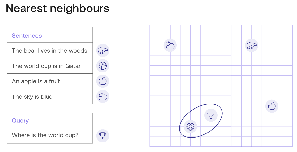
在此圖像中,所有句子都位於平面中的點。在視覺上,您可以確定查詢(由獎杯表示)最接近響應“世界杯在卡塔爾”,由足球表示。其他查詢(由雲、熊和蘋果表示)要遠得多。因此,語義搜索將返回“世界杯在卡塔爾”的響應,這是正確的響應。
但在我們進一步深入之前,讓我們實際使用現實生活中的文本嵌入在一個小數據集中進行搜索。以下數據集有四個查詢及其四個相應的響應。
Dataset:
Queries:
- Where does the bear live?
- Where is the world cup?
- What color is the sky?
- What is an apple?
Responses
- The bear lives in the woods
- The world cup is in Qatar
- The sky is blue
- An apple is a fruit
We can use the Cohere text embedding to encode these 8 sentences. That would give us 8 vectors of length 4096, but we can use some dimensionality reduction algorithms to bring those down to length 2. Just like before, this means we can plot the sentences in the plane with 2 coordinates. The plot is below.
我們可以使用 Cohere text embedding 來編碼這 8 個句子。這將給我們8個長度為4096的向量,但我們可以使用一些降維演算法將它們減少到長度為2。就像以前一樣,這意味著我們可以用 2 個座標在平面上繪製句子如下。

請注意,每個查詢最接近其相應的回應。這意味著,如果我們使用語義搜索來搜索對這 4 個查詢中的每一個的回應,我們將得到正確的回應。但是,這裡有一個警告。在上面的例子中,我們使用了歐幾里得距離,它只是平面中的距離。這也可以推廣到 4096 個條目的向量(使用勾股定理)。但是,這不是比較文本片段的想法方法。最常用和給出最佳結果的方式是相似性,我們將在下一節中研究。
使用 Similarity (相似度) 尋找最佳文本
相似性是一種判斷兩段文本是否相似或不同的方法。這使用 text embedding。此處是 sensentce embedding 而非 word embedding。如果您想了解相似性,請查看這篇文章。在本文中,描述了語義搜索中使用的兩種相似性:
-
點積 (dot product) 相似度
-
餘弦 (cosine) 相似度
現在,讓我們將它們視爲一個概念。相似度就是指定給兩個文本關係的一個數字,具有以下屬性:
- 一段文字與其自身的相似度是一個非常高的數字。
- 兩段非常相似的文本之間的相似度很高。
- 兩段不同的文本之間的相似度很小。
本文使用餘弦相似度,因爲它具有一個額外的屬性,即返回值介於 0 和 1 之間。一段文本與其自身之間的相似度始終為 1,並且相似度可以取的最低值為0(當兩段文本確實非常不同時)。
現在,為了語義搜索,所要做的就是計算查詢 query 與每對句子之間的相似度,並返回相似度最高的句子。舉個例子。下面是上述數據集中 8 個句子之間的餘弦相似度圖。

上圖的比例在右側給出。請注意以下特性:
- 對角線全是 1(因為每個句子與其自身的相似度為 1)。類似 graph 的 degree matrix?
- 每個句子與其相對應的回應之間的相似度約為 0.7。
- 任何其他兩個句子對之間的相似性都是較低的值。
這意味著,如果您要搜索 “What is an apple?” 這樣的查詢的答案,語義搜索模型會查看表格的倒數第二行,並找到到最接近的句子是 “What is an apple?” (相似度為 1)和 “An apple is a fruit” (相似度約為 0.7)。系統將從列表中刪除相同的查詢 (相似度為 1),因為它不想用相同於 query 來回應 (overfit or trivial)。因此,勝出的回應是 “An apple is a fruit”。這也是正確的回答。
這裡有一個隱藏的算法我們沒有提到,但是很重要:nearest neighbors algorithm (最近鄰算法。Again,是否暗示 graph!)。簡而言之,該算法找到數據集中某個點的最近鄰。在這個例子,算法找到了句子 “What is an apple?” 的最近鄰,而回應是句子 “An apple is a fruit”。
在下一節中,您將了解有關最近鄰的更多信息。
最近鄰算法 (Nearest Neightbors Algorithm) - 優點和缺點,以及如何解決它們
最近鄰是一種非常簡單且有用的算法,通常用於分類。 更一般地說,它稱為 k-nearest neighbors (knn),其中 k 是任意數字。 如果手頭的任務是分類,knn 將簡單地查看特定數據點的 k 最近鄰,並為數據點分配鄰居中最常見的標籤。 例如,如果手頭的任務是將一個句子分類為快樂或悲傷(情感分析),那麼 knn (k=3) 會做的是查看該句子的 3 個最近的鄰居(使用 embedding),並查看它們是否大多數(2)是快樂的或悲傷的。 這是它指定給句子的標籤。
knn 正是本文中為語義搜索所用的算法。 給定一個查詢,您在 embedding 中尋找最近的鄰居,這就是對查詢的回應。 在上例中,knn 效果很好。
然而,knn 並不是最快的算法。 原因是為了找到一個點的鄰居,需要計算該點與數據集所有其他點之間的距離,然後找到最小的一個。 如下圖所示,為了找到與 “where is the world cup?” 這句話最近的鄰居,我們必須計算 8 個距離,每個數據點都要算一次。

然而,當處理大量資料時,我們可以通過稍微調整算法以成為近似 knn 優化性能。 特別是在搜索方面,有幾項改進可以大大加快這個過程。 這是其中的兩個:
-
Inverted File Index (IVD):包括對相似文檔進行聚類,然後在最接近查詢的聚類中進行搜索。
-
Hierarchical Navigable Small World (HNSW):包括從幾個點開始,然後在那裡搜索。 然後在每次迭代中添加更多點,並在每個新空間中搜索。
多語言搜索
語義搜索的性能取決於 embedding 的能力。 因此 embedding 的能力可以轉化為語義搜索模型的能力,包含多語言的 embeddings。簡而言之,多語言 embedding 會將這些語言中任何文本映射到一個向量。 相似的多語言文本片段將被發送到相似的向量。 因此,可以使用任何語言的查詢(query)進行搜索,模型將搜索所有其他語言的答案。
下圖可以看到多語言 embedding 的示例。 Embedding 將每個句子映射到一個長度為 4096 的向量,就像在前面的示例中一樣,使用投影將這個向量映射到 2D 平面。

在此圖中,我們有 4 個英語句子,以及它們的西班牙語和法語直接翻譯。
English:
- The bear lives in the woods.
- The world cup is in Qatar.
- An apple is a fruit.
- The sky is blue.
Spanish:
- El oso vive en el bosque.
- El mundial es en Qatar.
- Una manzana es una fruta.
- El cielo es azul.
French:
- L’ours vit dans la forêt.
- La coupe du monde est au Qatar.
- Une pomme est un fruit.
- Le ciel est bleu.
正如圖中看到的,多語言模型將每個句子及其兩個翻譯非常靠近。
Embedding 和 Similarity 是否足夠? (不)
在本文中,您已經了解了當搜索模型由實體嵌入和基於相似性的搜索組成時,它是多麼有效。 但這就是故事的結局嗎? 不幸的是(或者幸運的是?)沒有。 事實證明,僅使用這兩個工具可能會導致一些意外。 幸運的是,這些是我們可以解決的事故。 這是一個例子。 讓我們稍微擴展一下我們的初始數據集,添加更多對世界杯問題的回答。 考慮以下句子。
Query: “Where is the world cup?”
Responses:
-
The world cup is in Qatar
-
The world cup is in the moon
-
The previous world cup was in Russia

當我們在上面的嵌入中定位它們時,正如預期的那樣,它們都很接近。 然而,最接近查詢的句子不是響應 1(正確答案),而是響應 3。這個響應(“上屆世界杯在俄羅斯”)是一個正確的陳述,並且在語義上接近問題,但它不是 問題的答案。 響應 2(“世界杯在月球上”)是一個完全錯誤的答案,但在語義上也接近查詢。 正如您在嵌入中看到的那樣,它非常接近查詢,這意味著像這樣的虛假答案很可能成為語義搜索模型中的最佳結果。
How do we fix this? There are many ways to improve search performance so that the actual response the model returns is ideal, or at least close to ideal. One of them is multiple negative ranking loss: Having positive pairs (query, response) and several other negative pairs (query, wrong response). Training the model to reward positive pairs, and punish negative pairs.
In the current example, we would take a positive (query, response) pair, such as this one:
(Where is the world cup?, The world cup is in Qatar.)
We would also take several negative (query, response) pairs, such as:
- (Where is the world cup?, The world cup is in the moon)
- (Where is the world cup?, The previous world cup was in Russia)
- (Where is the world cup?, The world cup is in 2022.)
By training the model to respond negatively to bad (query, response) pairs, the model is more likely to give the correct answer to a query.
Now the question is, how do we train the model to do this? This is a topic for a future article. Other search topics we’ll be exploring in the future are the following, so stay tuned!
- Semantic search, vector databases
- Multilingual semantic search
- Semantic search for long documents
- Re-ranking endpoint
- Billion-scale semantic search
- Semantic search over semi-structured data
- Bulk encoding embeddings


NLP Sematic Search and Classification Task
| Computer Vision | Voice | NLP | |
|---|---|---|---|
| Classification | dog, cat, very mature | sound scene | sentiment analysis, Q & A |
| Detection | bounding box | special sound, instrument | Q & A with start/end index |
| Recognition | Face recognition | Voice ID | Author ID? |
| Speech recognition | Figure caption? (img to text) | ASR (voice to text) | Translation? (text to text) or summary? |
| De-noise | De-noise | De-noise | Fill in empty |
| Super resolution | SR | SR | x (somewhat GAI) |
| MEMC | Inpainting, insert sequence | make voice more clear | x (somewhat GAI) |
| Chat | text to image | text to music/speech | Dialog, or generative AI (text-to text) |
Query, Key, and Value
The terms “query”, “key”, and “value” used in the attention mechanism have their origin in information retrieval and database management systems. The concept has been applied to Recommendation System and Transformer Model used in natural language processing.
在注意力機制中使用的查詢 (query)、鍵 (key) 和值 (value) 這些詞語,源自於資訊檢索 (information retrieval) 和數據庫管理系統 (database management system, e.g. SQL - Structured Query Language)。這個概念也被應用於自然語言處理中使用的推薦系統和Transformer模型中。
Information Retrieval and Database
In information retrieval, a “query” refers to the user’s request for information, while the “key” refers to the index used to retrieve relevant information from a database. The “value” is the actual information retrieved by the query using the key.
In natural language processing, the “query” can be seen as the input that the model receives, such as a sentence or a sequence of words. The “keys” and “values” are representations of the input used by the model to compute the attention scores. The “keys” can be seen as a set of learned representations of the input, while the “values” can be seen as the actual input features that are used to compute the output of the model.
In the attention mechanism, the “query” is used to compute the relevance of each “key” with respect to the input, and the “values” are used to compute the weighted sum of the relevant “values”. This process allows the model to focus on the most relevant parts of the input when generating the output.
Recommendation System
In a recommendation system, “query” typically refers to the current user or their current behavior, while “key” and “value” refer to the items in the system that the user might be interested in.
The idea is that the recommendation system uses the user’s behavior (query) to search for items in the system that match or are similar to the user’s interests (key), and then returns those items (value) as recommendations.
This is often done using techniques like collaborative filtering, content-based filtering, or a combination of both.
One example of a paper that discusses the use of “query”, “key”, and “value” in recommendation systems is “Collaborative Filtering for Implicit Feedback Datasets” by Yifan Hu, Yehuda Koren, and Chris Volinsky, which was published in the Proceedings of the 2008 Eighth IEEE International Conference on Data Mining.
Attention Mechanism in Transformer Model
The use of the terms “query”, “key”, and “value” in the context of attention mechanism originated from the seminal paper “Attention is All You Need” by Vaswani et al. (2017), which introduced the Transformer architecture. In this architecture, the attention mechanism is used to compute the contextual representation of each input element by attending to all other elements in the sequence.
In the Transformer, the attention mechanism is formulated as a mapping from a set of queries, represented by a sequence of vectors, to a set of values, represented by another sequence of vectors. The keys are also represented by a sequence of vectors, which are used to compute the attention weights between the queries and values. Specifically, the attention weights are computed by taking the dot product between the queries and keys, and then applying a softmax function to obtain a probability distribution over the values. The resulting attention weights are then used to compute the weighted sum of the values, which gives the contextual representation of each query.
The use of the terms “query”, “key”, and “value” in the attention mechanism reflects their respective roles in this process: the queries are the vectors that are being attended to, the keys are used to compute the attention weights, and the values are the vectors that are being attended over. This formulation has since become a standard way of describing attention mechanisms, and has been applied in a variety of neural network architectures for natural language processing, computer vision, and other domains.
Reference
Serrano, Luis. “What Are Word and Sentence Embeddings?” Context by Cohere. January 18, 2023.
https://txt.cohere.ai/sentence-word-embeddings/.
———. “What Is Semantic Search?” Context by Cohere. February 27, 2023.