我想用 matrix math 澄清一些觀念
A: m x n
B: n x p
A B = m x n . n x p = m x p highest rank 是 min(m, n, p)
Fully Connected
Reduce Dimension (1024->100): 例如 Computer Vision 分類問題 (最後幾層 mixed spatial and channel features)
A. 先考慮 1D case, Input 是 fixed (spatial) length (1024), Output 是 fixed category (100), feature size = 1
-
Input: 1024x1; Output 100x1; Weight: 100x1024 (非常自然!)
- Output (100x1) = Weight (100x1024) * Input (1024x1) => 1D vector = 2D matrix * 1D vector => rank ~ 100
- 不再贅述:或是 Input’ (1x1024) * Weight’ (1024x100) = Output’ (1x100)
- Input 是隨 content 變動的;Weights 是 trainable, 但是 train 完就 freeze; output 當然是隨 content 變動的
B. 1D case with input/output feature size 64. Input 是 (1024x64), Output (100x64), feature size = 64
- Input: 1024x64; Output 100x64; 這時的 Weight 是什麼???
- Output (100x64) = Weight (100x64)x(1024x64) * Input (1024x64) => 2D array = 4D tensor(!!!) * 2D array => rank ???
- (4D) fully connected (mixed) inter-inputs and intra-input (features) weights: 100x64 x1024x64 = input x output x (feature^2) = 419M! 所有的 inter-input 和 features 之間任意 mix! 非常大的 trainable weights and computations! 不實際
- 簡化 I:Only inter-inputs fully connected (mixed) weight, NO intra-input (feature) mix => weights 還是 100 x 1024 (x64?)! 所有的 feature 都 share 相同 weight.
- 簡化 II (NOT applicable in this case) : Only intra-input (features) fully connected (mixed) weight, NO inter-inputs mix. 就是 intra-input features 之間 mix, 而沒有 inter-inputs mix => weights 是 64x64! 所有的 input samples share 同樣的 weighs.
- 其實這就是 1x1 convolution! 所以這個操作也稱為 1x1 convolution!
- Convolution 的 input 和 output size 要相同!(最多差一個 padding). 對於 1x1 convolution, 不需要 padding, input = output dimension!
- 如果要改變 input and output size 除非再做 upsampling/downsampling!
- 1x1 convolution 在這個 case 無法使用,因為 input samples (1024) $\ne$ output samples (100)!
- (Caveat) 對於 transformer model: input sample 之間的 mix weights, 是由 attention block 達成! Feature 之間的 mix, 是從 MLP 1x1 convolution 達成!見下面。
- Input 是隨 content 變動的;Weights 是 trainable, 但是 train 完就 freeze; output 當然是隨 content 變動的
I/O Same Dimension (512->512): 生成式問題 (e.g. transformer encoder/decoder)
A. 先考慮 1D case, Input (token) 是 fixed length (512), Output (token) 是 fixed length (512), token embedding feature = 1
- Input: 512x1; Output 512x1; Weight: 512x512
- Output (512x1) = Weight (512x512) * Input (512x1)
- **實務上 NLP 的 input and output length 是變動的!!, CV 一般是固定的 **
- 所以才會有 attention layer 處理變動的部分, 而非用固定的 fully connected layer.
- Input 是隨 content 變動的;Weights 是 trainable, 但是 train 完就 freeze; output 當然是隨 content 變動的
B. 1D case with input/output feature size 768! Input (token) 是 (512x768), Output (token) (512x768), token embedding feature = 768!
- Input: 512x768; Output 512x768; 這時的 Weight 是什麼???
- Output (512x768) = Weight (512x768)x(512x768) * Input (512x768)
- (4D) fully connected (mixed) inter-inputs and intra-input (features) weights: 512x768 x512x768 = (token* feature)^2 = 155B! 所有的 inter-input 和 features 之間任意 mix! 非常大的 trainable weights and computations! 不實際
- 簡化 I (NOT applicable in this case) :Only inter-inputs fully connected (mixed) weight, NO intra-input (feature) mix => weights 是 512 x 512 (x768?)! 只是所有的 feature 都 share 同樣的 weight.
- 實務上 NLP 的 input and output length 是變動的!!, 固定的 512x512 weights 不實際
- 所以才會有 attention layer 處理變動的部分, 而非用固定的 fully connected layer.
- 簡化 II: Only intra-input (features) fully connected (mixed) weight, NO inter-inputs mix. 就是 intra-input features 之間 mix, 而沒有 inter-inputs mix => weights 是 768x768! 所有的 input samples share 同樣的 weighs.
- 其實這就是 convolution! 所以這個操作也稱為 1x1 convolution! Convolution 的 input 和 output 基本要相同!(最多差一個 padding). 對於 1x1 convolution, 不需要 padding, input = output dimension! 除非再做 upsampling/downsampling!
- (Caveat) 對於 transformer model: input sample 之間的 mix weights, 是由 attention block 達成! Feature 之間的 mix, 是從 MLP 1x1 convolution 達成!
- Input 是隨 content 變動的;Weights 是 trainable, 但是 train 完就 freeze; output 當然是隨 content 變動的
Multi-Layer Perceptron (MLP)
- 多半是 $\ge$ 2 layers, 如果只有 1 layer 基本就是 fully-connected layer
- 第一層稱為 hidden layer, node 數目多半大於或等於 input node. 可能 2 倍。
- 第二層如果是 output layer, node 數目一般小於 input node for 分類問題。等於 input for transformer token.
- 在 computer vision application, 多半是放在最後部分。feature size 已經被打包成 1.
- 例如: 1024x1 (input feature layer) -> 2048x1 (hidden layer) -> 100x1 (output)
(Kernel) Convolution layer
Convolution 其實蠻奇葩的。看起來像是 matrix multiplication. 但如果真的用 GEMM 做 convolution, 例如 GPU, 則會發生非常低的 utilization rate!! 這和 fully-connected layer 完全不同!
**為什麼 GEMM 會有非常低的 utilization rate? **
- 因為把 convolution 變成 matrix multiplication, 會得到 sparse matrix! 特別是 kernel 非常小 (e.g. 3x3) 的情況下。
- Kernel matrix 都是重複的 pattern
- 1D: Input: 256 x 1, Kernel: 3 x 1
- Kernel appends to Kernel matrix : 3 x1 => 256 x 258. (258 = 256 + 3 -1), 其中非 0 只有 3 x 258, 其他為 0. 另外非 0 的 258 列又是重複 pattern!!
- Output (258x1) = Expanded Kernel (258x256) * Input (256x1)
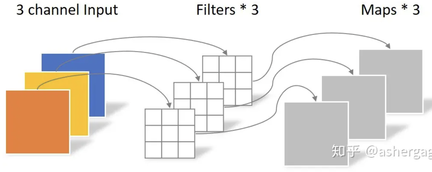
B. 假如 feature (channel-in, Cin) size 是 64
-
1D input + 1D channel: Input: 256 x 64, Kernel: 3 x 64
-
Kernel appends to Kernel matrix : 3 x 64 => 256 x 258 x 64, 其中非 0 只有 3 x 258, 其他為 0. 另外非 0 的 258 列是重複 pattern!!
- Output (258x64) = Expanded Kernel (258x64)x(256x64) * Input (256x64)
- (4D) fully connected (mixed) inter-inputs and intra-input (channel features) weights: (258x64) x (256x64)! 所有的 inter-input 和 features 之間任意 mix! 不過因為 kernel matrix 大多是 0, 只有對角線附近的元素 (kernel size, e.g., 3) 非 0 且重複,也就是 inter-input 只限制在 kernel size 的 mix. 所以 kernel weight parameters = (1(重複)x64) x (3(kernel 非0)x64) = 3 x 64 x 64! 就是 trainable parameters = 3 x 64 x 64. 也就是 kernel * Cin * Cout
- 簡化 I (depth-wise convolution):Only inter-inputs fully connected (mixed) weight, NO channel feature mix => weights 是 1(重複)x3(kernel)x64! 只是所有的 channel feature 都 share 同樣的 weight.
- 簡化 II (point-wise convolution):Only channel features fully connected (mixed) weight, NO inter-inputs mix. 就是 1x1 convolution. Channel features 之間 mix, 而沒有 inter-inputs mix => weights 是 64x64=Cin x Cout! 所有的 input samples share 同樣的 weighs.
- 這裡有一個 twist, 就是 output channel features 不一定要和 input channel feature 一樣, Cin x Cout!
- Input 是隨 content 變動的;Weights 是 trainable, 但是 train 完就 freeze; output 當然是隨 content 變動的
C. 假如 feature (2D input + channel-in, Cin) size 是 64
- 2D input + 1D Channel: Input: 256 x 256 x 64, Kernel: 3 x 3 x 64
- Kernel appends to Kernel tensor? : 3 x 3 x 64 => (256x258) x (256x258) x 64, 其中非 0 只有 3 x 3 x 258 x 258, 其他為 0. 另外非 0 的 258 列是重複 pattern!!
- Output (258x258x64) = Expanded Kernel (258x258x64)x(256x256x64) * Input (256x256x64)
- (4D) fully connected (mixed) inter-inputs and intra-input (channel features) weights: (258x64) x (256x64)! 所有的 inter-input 和 features 之間任意 mix! 不過因為 kernel matrix 大多是 0, 只有對角線附近的元素 (kernel size, e.g., 3x3) 非 0 且重複,也就是 inter-input 只限制在 kernel size 的 mix. 所以 kernel weight parameters = (1x1(重複)x64) x (3x3(kernel 非0)x64) = 3 x 3 x 64 x 64! 就是 trainable parameters = 3 x 3 x 64 x 64. 也就是 kernel * Cin * Cout
- 簡化 I (depth-wise convolution):Only inter-inputs fully connected (mixed) weight, NO channel feature mix => weights 是 3x3(kernel)x64! 只是所有的 channel feature 都 share 同樣的 weight.
- 簡化 II (point-wise convolution):Only channel features fully connected (mixed) weight, NO inter-inputs mix. 就是 1x1 convolution. Channel features 之間 mix, 而沒有 inter-inputs mix => weights 是 64x64=Cin x Cout! 所有的 input samples share 同樣的 weighs.
- 這裡有一個 twist, 就是 output channel features 不一定要和 input channel feature 一樣, Cin x Cout!
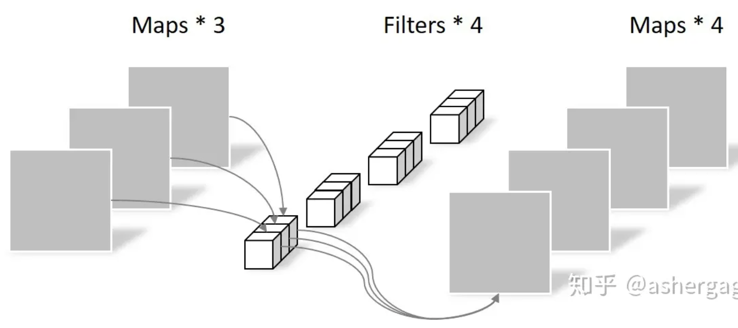
- 原來的 kernel size x Cin x Cout (full convolution) 變成 kernel size x Cin (depth-wise) + Cin x Cout (point-wise).
- 3x3x64x64 = 36.9K > 3x3x64x1 + 1x1x64x64 = 4.7K
- Input 是隨 content 變動的;Weights 是 trainable, 但是 train 完就 freeze; output 當然是隨 content 變動的
Convolution 雖然實際計算不會用 matrix multiplication. 當做理論用還是 OK.
Concatenate (Matrix Representation), Cout dimension!
Slice
Attention is all you need
NLP 的問題是 input text string 一般是變動的,例如:“Hello, world”, 或是 “This is a test of natural language processing!”
Input 是 text string, 切成 tokens ($\le$512). 儘量塞 sentence 或是 0 padding. 每個 token 是 768-dim (feature) vector. 也就是 (input) token embedding 是一個 arbitrary width ($\le$ 512) 2D matrix X. 最終希望做完 attention 運算還是得到同樣的 shape.
先看不好的方法 for Natural Language Porcessing
- 如果 input-output 是 inter-token 和 inter-feature 的 fully-connected network, 顯然不可行!
- 因為是一個 $(512\cdot 768)^2 = 154$ B weights,同時 computation 也要 154 T operation!
- Input 是變動的長度, 所以固定的 154B weights 無法得到不同 width 的結果。
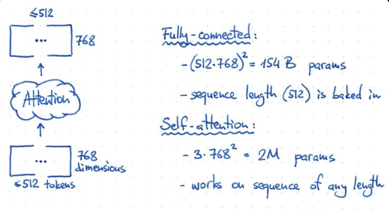
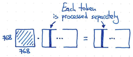
- 如果 input-output 只作用或處理在 embedding dimension (i.e shared weight for all input tokens!), 例如 1-dimension convolution, kernel 就是 1x768, channel length = 768. 假設 input 是 3-channel (e.g. RGB or KQV), parameter = 3 x 768^2 = 2M parameters. 顯然也不夠力。同時 each token 都是獨立處理,缺乏 temporal information!
Catch
- 我們需要找一個方法介於 fully connected model and 1-d convolution network!!!
- Fully connect network size: (512x768)^2 = 154B
- 1-dimension network size: (768x768) < 1M
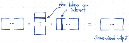
- 所以需要如同下面的方法!計算 $f(X) = X X^T X$. 假設 X 是 m x n -> (m x n) (n x m) (m x n) = m x n 得到和原來一樣的 shape!
- 此時 token 和 token 之間 interact, 但又不像 fully connected 這麼多 interaction!!! 這就是 attention 的原理!
- Rank = min(m, n)! 如果 width 很小,例如短句。或是 attention 範圍小。rank 就小。計算量就小,也避免 overfit!
- 問題是以下的方法,沒有任何 trainable parameter!!!!
如何引入 Trainable Parameter?
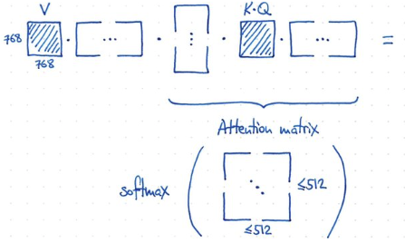
- 如何做到?非常容易! 重組 input 引入 V (value) matrix. 引入 K, Q matrix and similarity/attention matrix!!
- 使用 K, Q 計算 similarity matrix (512x512),then softmax for attention matrix. V 通過 attention matrix 得到 output!
- 因為 attention matrix 的遠小於 768! 所以有類似 low rank 的功效。
- V, K, Q 的 dimension:
- V: 768x768, K: 768x768, Q: 768x768. Total: 3 x (768x768)
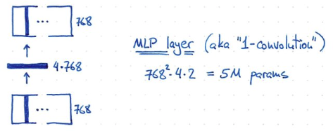
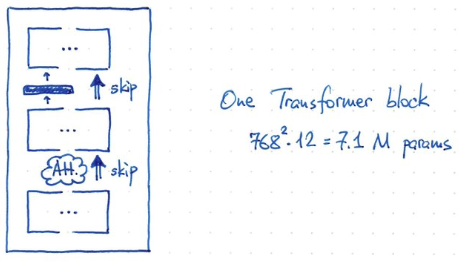
- 最後再加上一個 MLP layer. Hidden layer 的 dimension 是 4x768!, 所以 parameter = 768^2 x 4 x 2? = 5M parameters!
- 一個 transformer block 的 parameter = V,K,Q x 768^2 = 3 x 768^2 = 2M param + 5 M= 7.1 M parameters
- BERT 有 12 blocks, giving ~ 85M params (再加上 25M for token embedding, 512 x 768 = 0.39M??)
- GPT2 = ?
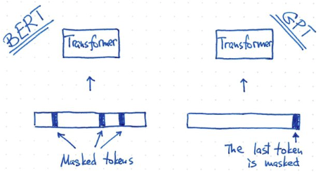
- BERT 和 GPT training 方式不同: BERT 使用 masked token. GPT 使用 predicted token.
Convolution is all you need
Input 大多是 256x256x3 (RGB) pixel (or 考量 data augmentation +/-16 pixel: 224x224 pixel ).
如果是 generative model, 例如 de-noise, de-blur, output 和 input dimension 一樣。
因爲不是分類問題,沒有用 fully-connected layer.
先看不好的方法 for Computer Vision
- Fully connected trainable parameter: (256x256x3)^2 = 38B! 雖然大力出奇蹟。但這只是小圖。如果是大圖 4K x 4K, 參數增加 16 倍。基本上 fully connected network 不 scalable!
- 如果是一次 depth-wise + point-wise trainable parameter = (256x256)^2 x 3 + 3x3 = 12.9B! 雖然比較小,還是非常大,not scalable!
可行的方法
三種方法:(1) convolution; (2) transformer; (3) hybrid.
(1) 第一種方法 convolution + hierarchy (down-sampling/up-sampling)
Kernel: 3x3, Cin = 3, Cout=64 => first layer: (shared) trainable weights = 3x3x3x64 = 1.7K!! 非常小。
- 但是 計算量 (要掃過所有圖區域) » trainable parameters. 就是計算量 dominate! 好處是 power efficiency 比較好,可以不用一直拿 weights.
- Kernel 小的缺點是 receptive field 非常小。需要 down-sampling and up-sampling 增加 receptive field! 但同時增加 channel depth (feature) 避免 loss information.
- 所以後面的 kernel trainable parameters 會增加: 3x3x512x1024 = 4.7M, 還在可控範圍!就算是 20 layers 也不過 ~80M parameters! 而且如果是 4K x 4K, parameter 是 linear 增加,而不是幾何增加!
- 如果還要更少 trainable weights, 可以用 depth-wise + point-wise (例如 MobileNet) => 3x3x512 + 1x1x512x1024 = 529K, 大約只有 4.7M 的 11%。
(2) 第二種方法 Vision Transformer (ViT)
如果是用 3x3 pixel 為一個單位 (patch),256x256 picture 就會有 7281 patches, 對於 transformer model 顯然太多。
ViT 使用 16x16 pixel 為一個 patch, 256x256 picture 就有 256 patches/tokens, 剛好可以給 transformer 使用!
如果一個 layer 是 7.1M parameter, 12 layers 就是 84M pixel. 好像還是在可接受範圍!
-
ViT 原理一樣!1-patch = 16x16x3 = 768 dimension. 224x224 image, 一共有 196 patches (<512 token).
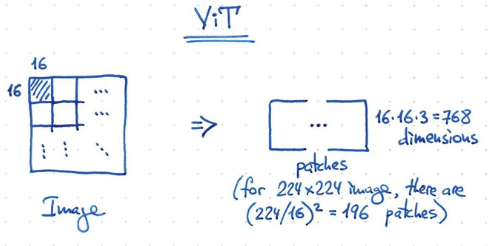
-
ViT 另一個簡化是使用 1-convolution 可以 work!! 也就是 shared weight!
ViT-22B
ViT-22B 是一個基于Transformer架構的模型,和原版ViT架構相比,研究人員主要做了三處修改以提升訓練效率和訓練穩定性。
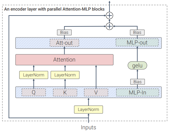
並行層(parallel layers)
ViT-22B並行執行注意力塊和MLP塊,而在原版Transformer中為順序執行。
Google 的 PaLM模型的訓練也採用了這種方法,可以將大模型的訓練速度提高15%,並且性能沒有下降。
query/key (QK) normalization
在擴展ViT的過程中,研究人員在80億參數量的模型中觀察到,在訓練幾千步之後訓練損失開始發散(divergence),主要是由於注意力logits的數值過大引起的不穩定性,導致零熵的注意力權重(幾乎one-hot)。
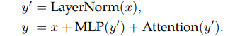
為瞭解決這個問題,研究人員在點乘注意力計算之前對Query和Key使用 LayerNorm
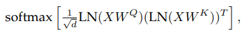
刪除QKV 投影和 LayerNorms 上的 bias
和PaLM模型一樣,ViT-22B從QKV投影中刪除 bias,並且在所有LayerNorms中都沒有 bias 和centering,使得硬件利用率提高了3%,並且質量沒有下降。
不過與PaLM不同的是,ViT-22B對(內部和外部)MLP稠密連接層使用了 bias,可以觀察到質量得到了改善,並且速度也沒有下降。
ViT-22B的編碼器模組中,嵌入層,包括抽取patches、線性投影和額外的 position embedding 都與原始ViT中使用的相同,並且使用多頭注意力pooling來聚合每個頭中的per-token表徵。
ViT-22B的patch尺寸為14×14,圖象的分辨率為224×224(通過inception crop和隨機水平翻轉進行預處理),一共有 224x224/(14x14)=16x16=256 patches。
(3) 第三種方法 Hybrid:
convolution 對於 local feature 效果不錯。但是 transformer 對於 global feature 很好。是否可以結合?
(A) 比如前幾層是用 convolution, 之後用 transformer!
(B) 或是 convolution 的 block 直接用 transformer block 替代或 vice versa
(C) 或是把 hierarchy (down-sampling) 用在 transformer.
(3C) SWIN Transformer
基本是利用 CNN 的 windows (local attention) + shifted windows + patch merge + hierarchy
只是先做 attention, 再用 local attention window + shifted attention windows (類似 CNN sliding windows!)
Vision Transformer應用到圖象領域主要有兩大挑戰:
- 視覺實體變化大,在不同場景下視覺Transformer性能未必很好
- 圖象分辨率高,像素點多,Transformer基于全局自注意力的計算導致計算量較大
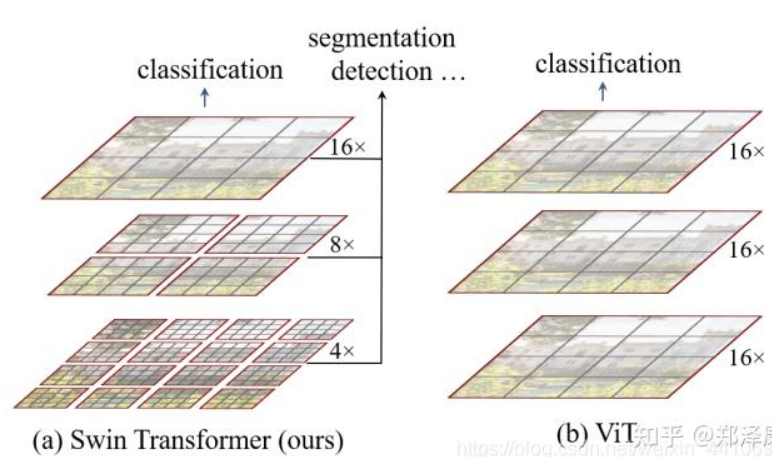
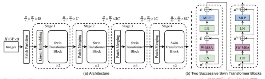
針對上述兩個問題,SWIN Transformer 提出了一種包含滑窗操作,具有”層級”設計的Swin Transformer。
其中滑窗操作包括不重疊的local window,和重疊的cross-window。將注意力計算限制在一個窗口中,一方面能引入CNN卷積操作的局部性,另一方面能節省計算量。
ViT 是 16x16 pixel/patch, 所以有 16x16 (256x256 pixels) patch.
SWIN 用更小的 pixel 為 patch, 這樣有很多的 tokens? (16倍) -> 使用更小的 (local) window attention.
Window attention + shifted window attention 取代 global attention!
用 patch merge 取代 pooling!
Math and figure:
- Input
####
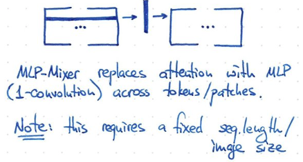
MLP is all you need
Masked MLP!!!!!!!!!!!!!!!!!!!!!!!!!!!
Patches are all you need
Math and figure:
https://arxiv.org/pdf/2201.09792.pdf
Music is all you need
Math and figure