Source
-
Efficient Memory Management for Large Language Model Serving with PagedAttention (arxiv.org)
-
Flash Attention with attention bias: https://zhuanlan.zhihu.com/p/567167376
-
Flash attention 2: https://tridao.me/publications/flash2/flash2.pdf
-
Flash Decoder: https://princeton-nlp.github.io/flash-decoding/
-
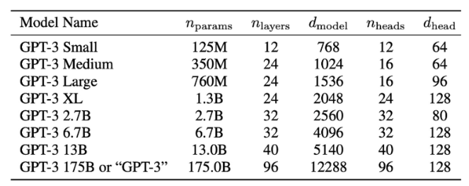
詳細的 GPT2/3 參數計算: https://www.lesswrong.com/posts/3duR8CrvcHywrnhLo/how-does-gpt-3-spend-its-175b-parameters
-
GPT3 原始 paper.
-
GPT2 原始 paper.
-
LLM1, https://finbarr.ca/how-is-llama-cpp-possible/
-
NLP(十七):从 FlashAttention 到 PagedAttention, 如何进一步优化 Attention 性能 - 知乎 (zhihu.com)
-
The KV Cache: Memory Usage in Transformers https://www.youtube.com/watch?v=80bIUggRJf4&ab_channel=EfficientNLP
Takeaway
- Attention block: KV cache memory management on (on-die) SRAM and the 1st memory (off-die memory).
- KV cache split, KV flash, KV decode
- dynamic cache
LLM Memory
LLM 的記憶體和 BW 包含兩個部分:需要存在 flash 和 app launch 是存在 DRAM 所占的記憶體。
- Static memory size and BW (只讀不寫):
- weight (參數量) x (precision) 和 input/output token length 以及 batch size 無關!
- 如果是 INT8, precision = 1 byte; INT4 (4W), precision = 0.5 byte; FP16 (16W), precision = 2 byte.
- Dynamic memory size and BW (又讀又寫): 和 input/output token length 以及 batch size 強相關!
- Training (16A16W): activation (中間激活), very big!
- Inference (Edge 4A16W or 4A8W): KV cache. 目的是減少 computation, 但會增加 bandwidth
參數量和靜態記憶體
Transformer 數學表示:
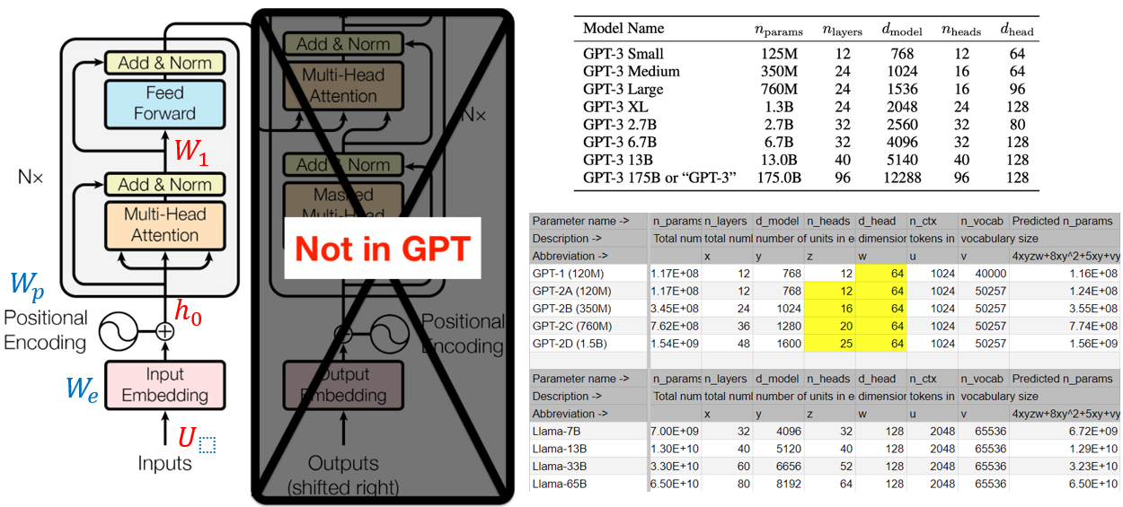
\[\begin{aligned} h_0 & =U W_e+W_p \\ h_l & =\text{transformer\_block}(h_{l-1}) \quad \forall \, l \in [1, n_{layers}] \end{aligned}\]where $U=\left(u_{-k}, \ldots, u_{-1}\right)$ is the context vector of tokens, $n$ is the number of layers, $W_e$ is the token embedding matrix, and $W_p$ is the position embedding matrix. \(\begin{aligned} \text{MultiHead}(Q, K, V) & =\text{Concat}\left(\text{head}_1, \ldots, \text{head}_{n_{heads}}\right) W^O \\ \text { where \quad head}_i & =\text {Attention}\left(Q W_i^Q, K W_i^K, V W_i^V\right) \end{aligned}\) Where the projections are parameter matrices $W_i^Q \in \mathbb{R}^{d_{\text {model }} \times d_k}, W_i^K \in \mathbb{R}^{d_{\text {model }} \times d_k}, W_i^V \in \mathbb{R}^{d_{\text {model }} \times d_v}$ and $W^O \in \mathbb{R}^{h d_v \times d_{\text {model }}}$. Exhibit C: An unnamed equation on page 5 in the original transformer paper. In the terminology of GPT, $d_k=d_v=d_{h e a d}$, and $h=n_{\text {heads }}$ \(\operatorname{FFN}(x)=\max \left(0, x W_1+b_1\right) W_2+b_2\) 幾實際例子
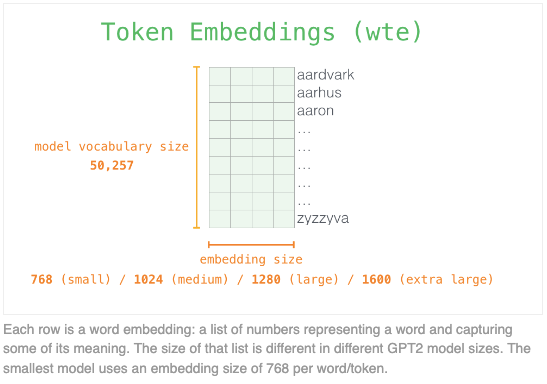
Embedding - 參數 $W_{e}$ : $n_{vocab} \times d_{model}$,$W_{p}$ : $n_{ctx} \times d_{model}$
-
$U$ 的大小是 ($n_{ctx} \times n_{vocab}$),$W_{e}$ 的大小是 ($n_{vocab} \times d_{model}$),$W_{p}$ 的大小是 ($n_{ctx} \times d_{model}$)。
-
Vocabulary size ($n_{vocab}$) 是 50257。乍看很大,但是 one-hot,也就是 $U$ 的 element 只有 0 或 1. $W_e$ 基本就是一本字典,每一個 vocabulary in 50257 都對應一個 embedding of vector length $d_{model}$.
-
所有的 models 都用同一個 context window, 其大小 $n_{ctx} = 2048$ tokens. 這個 context window size 決定這個 model 的記憶範圍。
-
$h_0$ 的大小是 $(n_{ctx} \times d_{model})$。
Attention Block - 參數 $W_i^{Q,K,V}$ : $3 d_{model} d_{head} n_{head} = 3 (d_{model})^2$,$W^{O} = (d_{model})^2$ , total = $4 (d_{model})^2$, need to add 4 d bias? yes => $4 (d_{model})^2 + 4 d_{model}$
- $Q, K$ 都是 $h_0$, 大小都是 $(n_{ctx} \times d_{model})$
- $V$ 是 output shifted right, 因爲 FFN 保持 input size 到 output size, 所以大小也是 $(n_{ctx} \times d_{model})$
- 對於 MultiHead attention, 每一個 head 的長度是 $d_{head}$,而且 $d_{model} = d_{head} \times n_{heads}$
- 每一個 head 都是三個矩陣乘法,$Q W_i^Q, K W_i^K, V W_i^V$,每個矩陣乘法大小是 $(n_{ctx} \times d_{model})\times (d_{model}\times d_{head})$,所以 head output 大小是 $n_{ctx}\times d_{head}$。但是因爲有 $n_{head}$ 而且 concat 在一起再做一次矩陣乘法 with $W^O$,所以 $\text{MultiHead}(Q,K,V)$ 的大小是 ($n_{ctx}\times d_{model}$).
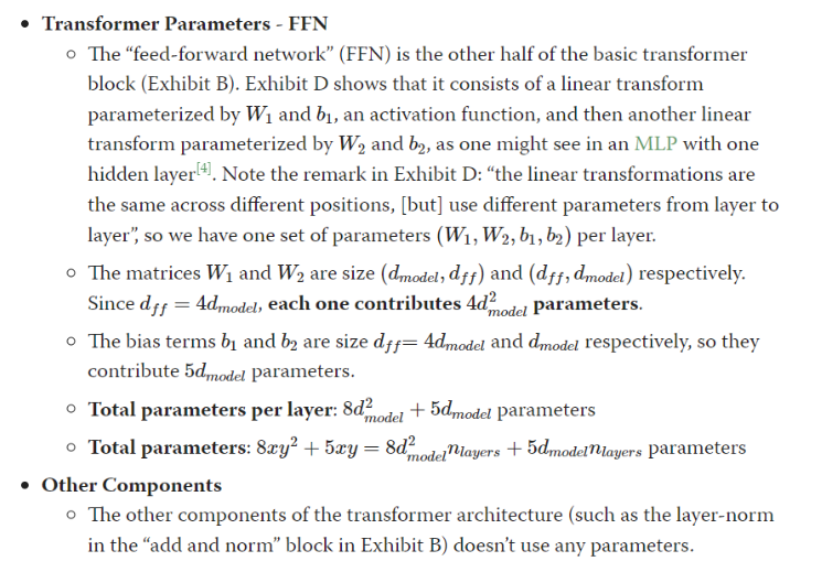
Feed-Forward Network (FFN) - 參數 $W_{1,2}: 2\times d_{model} \times 4 d_{model} = 8 (d_{model})^2$ and $b_{1,2} = 5 d_{model}$ => $8 (d_{model})^2 + 5 d_{model}$
- Feed-forward network (FFN) 的 input 和 output 都一樣大小 $d_{model}$, 而且只有一層 hidden layer, $d_{ff} = 4 d_{model}$. 這一層 hidden layer 和 input 以及和 output 都是 fully connected network. 所以兩個的參數量都是 $d_{model} \times 4 d_{model}$ 再加上兩個 bias $4 d_{model} + 1 d_{model} = 5 d_{model}$.
- FFN 的最後大小和 input 一樣: ($n_{ctx}\times d_{model}$).
Layer Norm - 參數 $\gamma, \beta$ : $4d_{model}$
elf-attention块和MLP块各有一个layer normalization,包含了2个可训练模型参数:缩放参数 $\gamma$ 和平移参数 $\beta$,形状都是 [ℎ] 。2个layer normalization的参数量为 4ℎ 。
GPT/Llama 總參數量:
一層的 transformer block:
$W_i^{Q,K,V},W_{1,2}, b_{1,2} = 4(d_{model})^2+4 d_{model} + 8(d_{model})^2 + 5 d_{model} + 4d_{model} = 12(d_{model})^2 + 13 d_{model}$
$n_{layers}$ 多層以及加上 $W_e, W_p$ 總參數量:
$n_{vocab}d_{model}+n_{ctx}d_{model}+n_{layers} \times (12 (d_{model})^2+ 13 d_{model})$
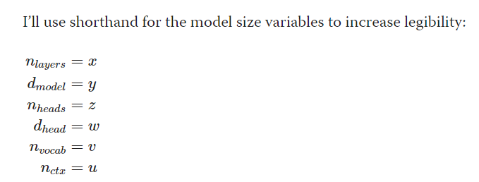
Variable 縮寫
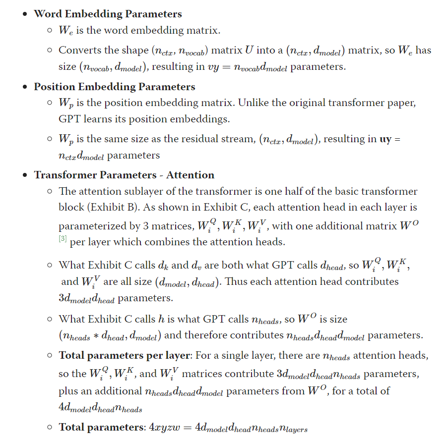
所以總共的參數有:$vy+uy+4xyzw+8xy^2 + 13xy = y(v + u) + x (4yzw+8y^2+13y)$.
一般 $y = zw$ 所以也可以寫成 $y(v+u) + x (12y^2+13y)$.
這也是上式: $P= d_{model} \cdot (n_{vocab}+n_{ctx})+n_{layers} \cdot (12 (d_{model})^2+ 13 d_{model})$
- 注意參數量 (不含 $W_p$) 和 token length 也和 batch 無關。這和 activation 不同!!!
- 如果使用相對位置編碼,例如 RoPE (Llama) or ALiBi, 不包含可訓練的參數,$W_p$ 可以忽略。
- 另一種寫法是 $P = Vh + l (12 h^2 + 13 h)$

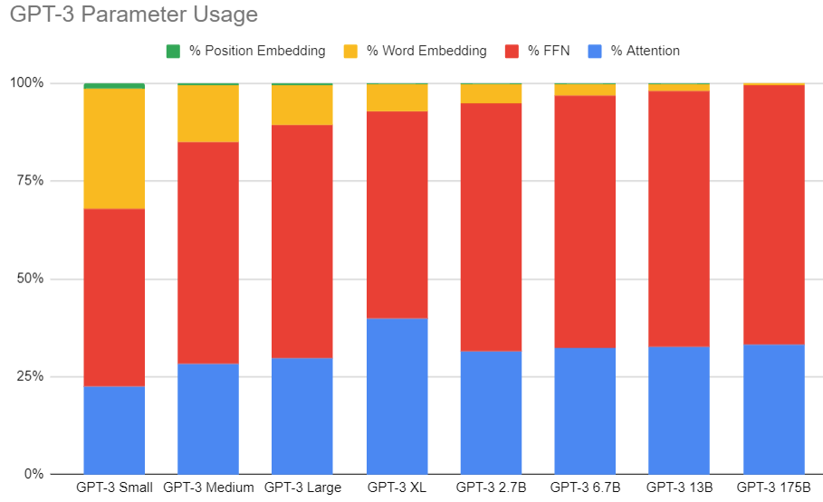
GPT3 參數量比例
下圖以各種不同大小 GPT-3 的參數比例圖示如下。其中佔大部分 60%+ 的參數是 FFN, attention 大約佔 30%+.
其他的參數 embedding matrix 和 position encoding 只佔個位數比例。 FFN 一般可以使用 low-precision 例如 INT4 以減少 memory footprint.
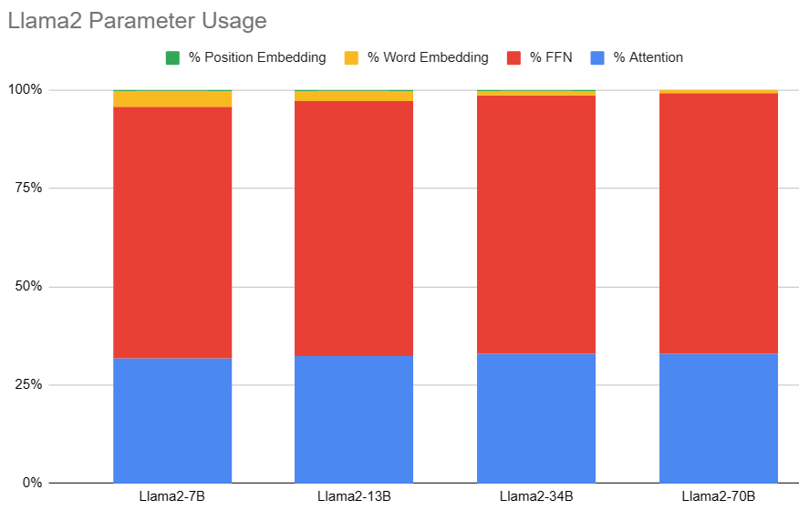
Llama2 參數量比例
- Position embedding 可以忽略
- FFN 基本佔 65%; Attention 基本佔 32%
接下來分析 activation, 也就是動態記憶體
中間激活 (Activation) 記憶體分析 (主要是 training 才需要存 activations) 16A16W
- Inference 只存 KV cache (attention 的部分)
除了模型参数、梯度、优化器状态外,占用显存的大头就是前向传递过程中计算得到的中间激活值了,需要保存中间激活以便在后向传递计算梯度时使用。这里的激活(activations)指的是:前向传递过程中计算得到的,并在后向传递过程中需要用到的所有张量。这里的激活不包含模型参数和优化器状态,但包含了dropout操作需要用到的mask矩阵。
在分析中间激活的显存占用时,只考虑激活占用显存的大头,忽略掉一些小的buffers。比如,对于layer normalization,计算梯度时需要用到层的输入、输入的均值和方差。输入包含了 $bsh$ 个元素,而输入的均值和方差分别包含了 bs 个元素。由于 ℎ 通常是比较大的(千数量级),有 bsh≫bs 。因此,对于layer normalization,中间激活近似估计为 bsh ,而不是 bsh+2bs 。
大模型在训练过程中通常采用混合精度训练,中间激活值一般是float16或者bfloat16数据类型的。在分析中间激活的显存占用时,假设中间激活值是以float16或bfloat16数据格式来保存的,每个元素占了2个bytes。唯一例外的是,dropout操作的mask矩阵,每个元素只占1个bytes。在下面的分析中,单位是bytes,而不是元素个数。
每个transformer层包含了一个self-attention块和MLP块,并分别对应了一个layer normalization连接。
Self attention
b = batch 在 training 時,會有 batch input, 在 inference 是 batch = 1 for ChatGPT model.
s = n_ctx (input tokens)
h = d_model ( = num_head * d_head)
- 此處考慮 batch size, 因爲 training.
- ChatGPT inference 的 batch size = 1. 以及在某些 network (大小網絡) batch size > 1 可以加速。
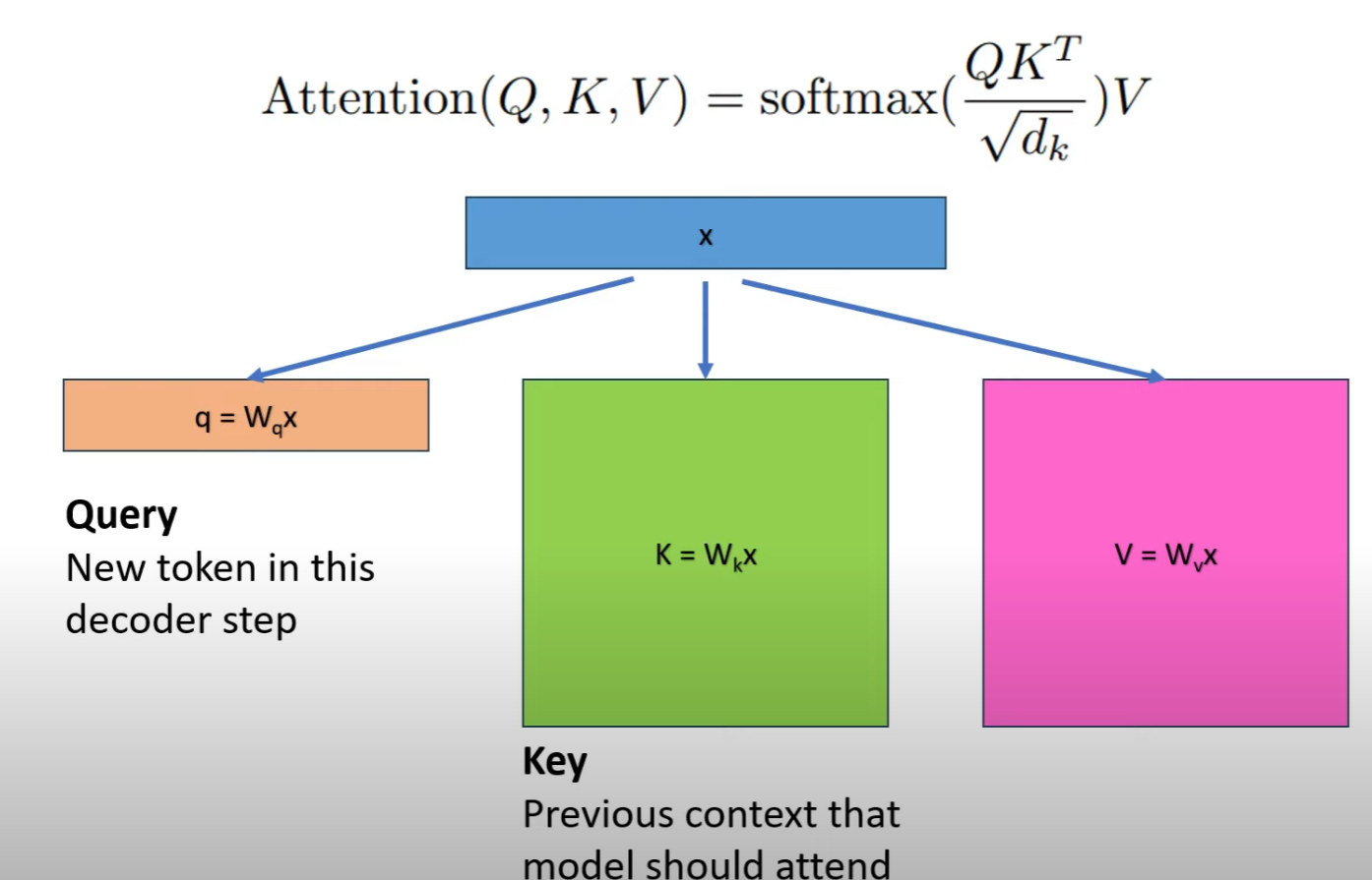
K, Q, V: Mapping Matrix : $Q = x_{in} W_Q,K = x_{in} W_K, V = x_{in} W_V$
- input 和 output shape [b, s, h] x [h, h] –> [b, s, h]
- Input activation 的量是: $p b s h$, p 是 precision, 如果是 FP16, p 是 2 個 byte.
QK: Attention matrix $x_{out} = \text{softmax}\left( \frac{Q K^T}{\sqrt{h}}\right) \cdot V \cdot W_O + x_{in}$
- 此處要考慮 multi-heads, 因此把 3D 的 Q, K, V [b, s, h] reshape 成 4D [b, head_num, s, per_head_hidden_size] where h = d_model = head_num * per_head_hidden_size
- $Q K^T$ 矩陣的 input 和 output [b, head_num, s, per_head_hidden_size] x [b, head_num, per_head_hidden_size, s] –> [b, head_num, s, s]
- Input activation 的量是: $2 p b s h$,
Softmax $x_{out} = \text{softmax}\left( \frac{Q K^T}{\sqrt{h}}\right) \cdot V \cdot W_O + x_{in}$
- input 和 output shape 都是: [b, head_num, s, s]
- Input activation 的量是: $p b s^2 a$,
- 计算完 softmax 函数后,会进行dropout操作。需要保存一个mask矩阵,mask矩阵的形状与 softmax 相同,占用显存大小为 $ b s^2 a$。Make 只需要 1 byte, 不用乘 p.
Score $x_{out} = \text{softmax}\left( \frac{Q K^T}{\sqrt{h}}\right) \cdot V \cdot W_O + x_{in}$
- input 和 output shape 都是: [b, head_num, s, s] x [b, head_num, s, per_head_hidden_size] –> [b, head_num, s, per_head_hidden_size]
- Input activation 的量是: $p b s^2 a + p b s h$,
Output Mapping $x_{out} = \text{softmax}\left( \frac{Q K^T}{\sqrt{h}}\right) \cdot V \cdot W_O + x_{in}$
- input 和 output shape 都是: [b, s, h] x [h, h] –> [b, s, h]
- Input activation 的量是: $p b s h$, 再加上一個 dropout $b sh$, total $(p+1) b s h$
Self-Attention 的 activation
$p b s h + 2 p b s h + p b s^2 a + p b s^2 a + b s^2 a + p b sh + (p+1)bsh = (5p+1) b s h + (2p+1) b s^2 a$
MLP
\[x_{mlp} = f_{gelu} (x_{out} W_1) W_2 + x_{out}\]- 第一個 FC (W1),
- Input activation 的量是: $p b s h$
- GELU 需要保存輸入:$4p b s h$
- 第二個 FC (W2),矩陣乘法的輸入和輸出 [b, s, 4h] x [4h, h] –> [b, s, h]
- Input activation 的量是: $4p b s h$
- 最後有一個 dropout, 需要保存 mask 矩陣, 大小是 $bsh$
MLP 的 activation
$(9p+1) b s h $
另外,self-attention块和MLP块分别对应了一个layer normalization。每个layer norm需要保存其输入,大小为 $pbsh$ 。2个layer norm需要保存的中间激活为 $2pbsh$.
综上,每个transformer层需要保存的中间激活占用显存大小为 $(16p+2) bsh + (2p+1) b s^2 a$ 。对于 $l$ 层transformer模型,还有embedding层、最后的输出层。embedding层不需要中间激活。总的而言,当隐藏维度 ℎ 比较大,层数 $l$ 较深时,这部分的中间激活是很少的,可以忽略。因此,对于 $l$ 层transformer模型,中间激活占用的显存大小可以近似为 $((16p+2)bsh + (2p+1) b s^2 a)*l$ 。
4.1 对比中间激活与模型参数的显存大小
在一次训练迭代中,模型参数(或梯度)占用的显存大小只与模型参数量和参数数据类型有关,与输入数据的大小是没有关系的。优化器状态占用的显存大小也是一样,与优化器类型有关,与模型参数量有关,但与输入数据的大小无关。而中间激活值与输入数据的大小(批次大小 $b$ 和序列长度 $s$)是成正相关的,随着批次大小 $b$和序列长度 $s$的增大,中间激活占用的显存会同步增大。当我们训练神经网络遇到显存不足OOM(Out Of Memory)问题时,通常会尝试减小批次大小来避免显存不足的问题,这种方式减少的其实是中间激活占用的显存,而不是模型参数、梯度和优化器的显存。
Example Llama-7B (16A16W)
以 Llama2-7B 爲例。
| 模型名 | 参数量 | 层数, l | 隐藏维度, h | 注意力头数 a |
|---|---|---|---|---|
| Llama2-7B | 7B | 32 | 4096 | 32 |
| Llama2-13B | 13B | 40 | 5120 | 40 |
| Llama2-33B | 33B | 60 | 6656 | 52 |
| Llama2-70B | 70B | 80 | 8192 | 64 |
Llama2 的模型参数量为7B,占用的显存大小为 (FP16) 7Bx2 = 14GB 。假設 activation 是 FP16.
假設 Llama2 的序列长度 $s$ 为 2048 。对比不同的批次大小 $b$ 占用的中间激活:
当 b=1 时,中间激活占用显存为 $(34bsh+5bs^2 a)*l$ byte ≈30.6GB ,大约是模型参数显存的2.2倍。
假設 Llama2 的序列长度 $s$ 为 4096 。对比不同的批次大小 $b$ 占用的中间激活:
当 b=1 时,中间激活占用显存为 $(34bsh+5bs^2 a)*l$ byte ≈104.2GB ,大约是模型参数显存的7.4倍。
Example GPT3-175B (16A16W)
以GPT3-175B为例,我们来直观地对比下模型参数与中间激活的显存大小。GPT3的模型配置如下。我们假设采用混合精度训练,模型参数和中间激活都采用float16数据类型,每个元素占2个bytes。
| 模型名 | 参数量 | 层数, l | 隐藏维度, h | 注意力头数 a |
|---|---|---|---|---|
| GPT3 | 175B | 96 | 12288 | 96 |
GPT3的模型参数量为175B,占用的显存大小为 2×175B = 350GB 。GPT3模型需要占用350GB的显存。
GPT3的序列长度 $s$ 为 2048 。对比不同的批次大小 $b$ 占用的中间激活:
当 b=1 时,中间激活占用显存为 $(34bsh+5bs^2 a)*l=275,414,777,856$ byte ≈275GB ,大约是模型参数显存的0.79倍。
当 b=64 时,中间激活占用显存为 $(34bsh+5bs^2 a)*l=17,626,545,782,784$ byte ≈17.6TB ,大约是模型参数显存的50倍。
当 b=128 时,中间激活占用显存为 $(34bsh+5bs^2 a)*l=35,253,091,565,568$ byte ≈35.3TB ,大约是模型参数显存的101倍。
可以看到随着批次大小 $b$ 的增大,中间激活占用的显存远远超过了模型参数显存。通常会采用激活重计算技术来减少中间激活,理论上可以将中间激活显存从 O(n) 减少到 O($\sqrt{n}$) ,代价是增加了一次额外前向计算的时间,本质上是“时间换空间”。
Memory BW for Training
假設 on-die 的 SRAM 很小 (<20MB), 所以一定要用外部的 DRAM (HBM 或是 DDR) 存儲參數和中間激活。
在 training 的 forward path 要讀一次參數,讀一次中間激活,和寫一次中間激活。
在 training 的 backward path 也要讀一次參數,讀一次中間激活,和寫一次中間激活。
也就是 Memory BW = 2 x 參數 (讀) + 2 x 激活 (讀) + 2 x 激活 (寫)
Example Llama-7B
当 b=1 时 : 14GB x 2 + 30.6GB x 4 = 150.4GB, 也就是每個 token (還是 2048 tokens?) 需要這麽大 memory BW.
KV Cache for Inference (主要用於推理)
KV Cache 的主要工作是減少 computation! 不是 DRAM BW reduction! 剛好相反,KV cache 會增加 DRAM bandwidth.
本质上是“空间换時间”。
- 0-cache 每次都要從 DRAM 讀 parameter 計算所有 output token:
- DRAM BW = parameter size x output token/sec
- Computation = 2 x parameter size TOPS
- KV cache 假設 internal SRAM = parameter size + KV cache: 理論上 DRAM access 只需要一次?
- DRAM BW = parameter size x output token/sec + KV cache size x 6 x output token/sec?
- DRAM BW / token = parameter size + KV cache size x 6 (讀幾次? 寫幾次?)
- Computation = ?? TOPS (減少多少?) 見下文
是否可能 “時間換空間”? On-die 7GB 或是 3.5GB SRAM,不可能!
在推断阶段,transformer模型加速推断的一个常用策略就是使用 KV cache。一个典型的大模型生成式推断包含了两个阶段:
- 预填充阶段:输入一个prompt序列,为每个transformer层生成 key cache和value cache(KV cache)。
- 解码阶段:使用并更新KV cache,一个接一个地生成词,当前生成的词依赖于之前已经生成的词。
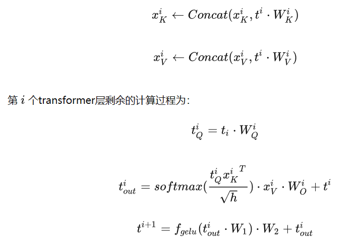
第 $i$个transformer层的权重矩阵为 $W_Q^i, W_K^i, W_V^i, W_O^i, W_1^i, W_2^i$。
其中 self-attention 的 4 個權重矩陣 $W_Q^i, W_K^i, W_V^i, W_O^i \in R^{h \times h}$。
并且MLP块的2个权重矩阵 $W_1^i \in R^{h \times 4h}, W_2^i \in R^{4h \times h}$。
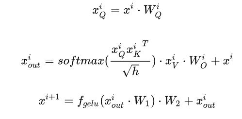
预填充阶段
假设第 $i$个transformer层的输入为 $x^i$ ,self-attention块的key、value、query和output表示为 $x_K^i, x_V^i, x_Q^i, x_{out}^i$ 其中 $x_K^i, x_V^i, x_Q^i, x_{out}^i \in R^{b\times s\times h}$。
Key cache 和 value cache 的計算過程為
$x_K^i = x^i \cdot W_K^i$
$x_V^i = x^i \cdot W_V^i$
第 $i$ 個 transformer 層剩餘的計算過程為
解码阶段
给定当前生成词在第 $i$ 个transformer层的向量表示为 $t^i \in R^{b \times 1 \times h}$. 推理計算分兩部分:更新 KV cache 和計算第 $i$ 個 transformer 層的輸出。
更新 key cache 和 value cache 的計算過程如下:
KV cache的显存占用分析
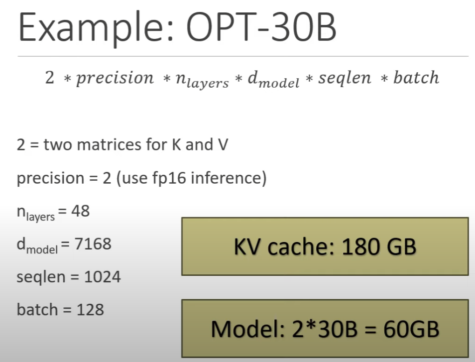
假设输入序列的长度为 $s$,输出序列的长度为 $n$,以float16来保存KV cache,那么KV cache的峰值显存占用大小为 $b(s+n)hl2*2 = 4blh(s+n)$。这里第一个2表示K/V cache,第二个2表示float16占2个bytes。
- Training 的中間激活時 : $34 blsh + 11 b l s^2 a$, KV cache 只存了 attention 中的 K and V 部分,有包含 score?
- Model 參數量是 $12 l h^2$ (和 b, s 無關!), 假設是 16-bit, Model 内存是 $24 l h^2$
- 假設 inference $b=1$ (這不一定是對的,在 speculative decode, 大 model 的 $b > 1$): KV cache : $4 blh (s+n)$. KV cache / model parameter ~ $b (s+n) / 6 h$! 對於 long context, $s + n$ 可能會大於 $h$!! $s$ 就是 $n_{ctx}$, $h$ 就是 $d_{model}$
- 以 Llama2-7B 爲例, $h = 4096$, 但是 $n_{ctx} 最大也有 4096$!
Example Llama2 (4A16W)
以 Llama2-7B 爲例。
| 模型名 | 参数量 | 层数, l | 隐藏维度, h | 注意力头数 a | Context s |
|---|---|---|---|---|---|
| Llama2-7B | 7B | 32 | 4096 | 32 | 4096 |
| Llama2-13B | 13B | 40 | 5120 | 40 | 4096 |
| Llama2-33B | 33B | 60 | 6656 | 52 | 4096 |
| Llama2-70B | 70B | 80 | 8192 | 64 | 4096 |
Llama2 的模型参数量为7B,占用的显存大小为 (INT8) 7Bx2 = 7GB 。假設 activation 是 FP16.
假設 Llama2 的序列长度 $s$ 为 2048 。对比不同的批次大小 $b$ 占用的中间激活:
当 b=1 时,KV cache 占用显存为 $(4bsh)*l$ byte ≈1GB ,大约是模型参数显存的15%。
假設 Llama2 的序列长度 $s$ 为 4096 。对比不同的批次大小 $b$ 占用的中间激活:
当 b=1 时,KV cache 占用显存为 $(4bsh)*l$ byte ≈2.1GB ,大约是模型参数显存的31%。
如果 model 是 4-bit (4W16A) 7Bx0.5 = 3.5GB, 更糟糕: KV cache 佔的比例 double.
Example GPT3-175B (8A16W)
以GPT3-175B为例,我们来直观地对比下模型参数与中间激活的显存大小。GPT3的模型配置如下。我们假设采用混合精度训练,模型参数和中间激活都采用float16数据类型,每个元素占2个bytes。
| 模型名 | 参数量 | 层数, l | 隐藏维度, h | 注意力头数 a |
|---|---|---|---|---|
| GPT3 | 175B | 96 | 12288 | 96 |
GPT3的模型参数量为175B,占用的显存大小为 1×175B = 175GB for inference。
GPT3的序列长度 $s$ 为 2048 。对比不同的批次大小 $b$ 占用的中间激活:
b=1 ,输入序列长度 s=2048, 中间激活占用显存为 $(4bsh)*l$ byte ≈9.7GB ,大约是模型参数显存的 5.6%。
b=64 ,输入序列长度 s=512 ,输出序列长度 n=32 ,则KV cache占用显存为 $4blh(s+n) = 164 GB$,大约是模型参数显存的 1 倍。
The KV Cache: Memory Usage in Transformers
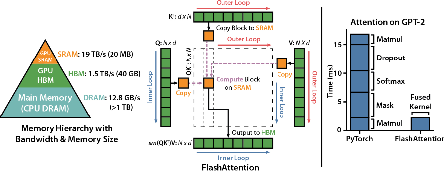
GPU Memory Hierarchy
先比較一下常見的 edge device memory hierarchy.
| Compute Core | SRAM Size/BW | 1st Mem Size/BW | 2nd Mem Size/BW | |
|---|---|---|---|---|
| A100 | (FP16) 312 TOPS Tensor |
20MB / 19TB/s | (HBM2?) 40GB / 1.5TB/s | CPU DRAM > 1TB / 12.8GB/s |
| Smartphone | (INT8) 40 TOPS | 8MB / ?? | (LP5-8500, 64bit) 12GB / 50GB/s | Flash, 512TB / 1GB/s? |
| RTX4070TI | 7680 Shader 184 Tensor (FP32) 40 TOPS |
(G6X, 192bit) 12GB / 504GB/s | NA |

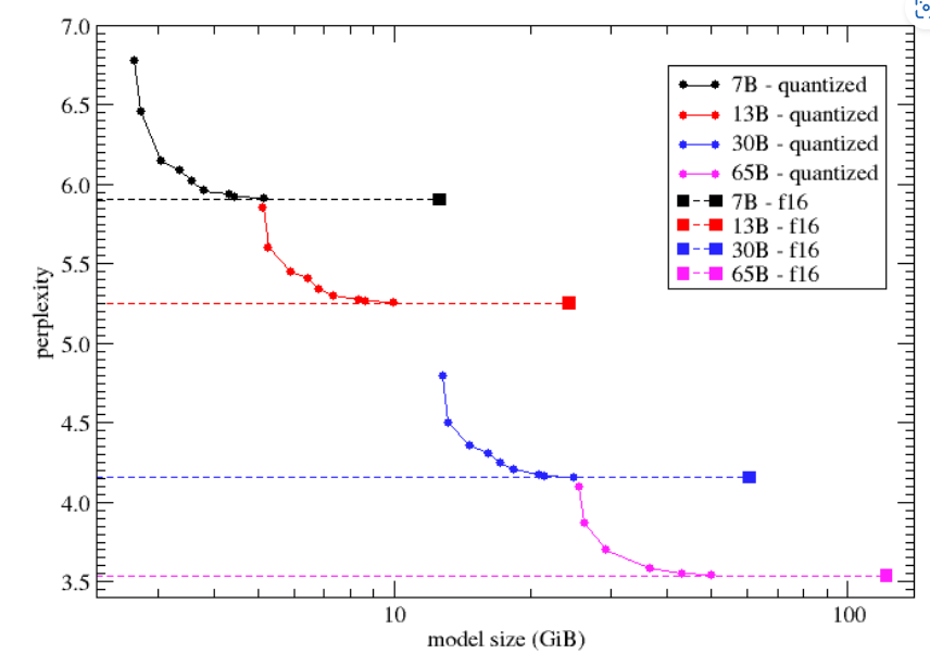
Quantization vs. Model Size
####
Attention is what you need, Memory is the Bottleneck
Attention 已經是必備的 core network. 相較於 CNN, attention 最大的問題是 memory bandwidth.
主要在計算 K, Q 的 correlation, 以及 softmax. 以下是 GPT1/2/3 的參數。
下圖應該畫錯了! GPT 應該是 decoder only (右邊)。所以對應的方塊圖是沒有 encoder (左邊),只有 decoder (右邊)。所以打叉的地方相反。BERT 才是 encoder only (左邊)。不過兩者的架構非常類似。不過 decoder only 架構 output 會 shift right 再接回 input, 稱爲 auto-regression.
算力估計 TOPS:
我們先用最直觀的方法計算。
假設計算一個 output token 需要把所有的參數 $P$ 都用過一次。如果 output token rate 是 $B$ token/sec.
則所需要的算力 (只有 matrix multiplication, 不包含 softmax, layer norm, etc.) 是 $2 \cdot P \cdot B$. 這裏的 2 是加法和乘法。同時假設 inference batch size = 1. 這對一般 edge device 是合理的。
所以算力就是 $2 P B$.
-
如果是小 7B model, 同時 B = 20 token/sec, 就是 2x7Bx20 = 280 GOPS. 看起來好像不大。一般是 softmax 的算力佔大部分。
-
如果是跑大的模型例如 33B, 同時 B = 100 token/sec, 2 x 33B x 100 = 6.6 TOPS.
Refine:
DRAM 頻寬估計:
同樣用直觀估計頻寬,假設每個參數都要讀出 DRAM, 先忽略中間值, i.e. 每層的 input/output (activation),也要寫入和讀出 DRAM. 另外引入一個參數 $n_{byte}$ 代表每個參數使用的 byte 數目。
| $n_{byte}$ | |
|---|---|
| FP32 | 4 |
| FP16 | 2 |
| INT8 | 1 |
| INT4 | 0.5 |
$BW = n_{byte} \cdot P \cdot B $
此處沒有 2 因爲加法和乘法只需要一次進出 DRAM.
- 7B model, B = 20 token/sec, INT4: 0.5 byte/token x 7G x 20 token/sec = 70 GB/sec.
- 33B model, B = 100 token/sec, INT4: 0.5 byte/token x 33G x 100 token/sec = 1650 GB/sec
常見系統 DRAM 頻寬
| DRAM Type | DRAM 大小 | DRAM 頻寬 | TOPS | Rate | |
|---|---|---|---|---|---|
| H100 | HBM | GB | GB/sec | ||
| A100 | HBM | 40-80 GB | 1935 GB/sec | 312@INT8 | |
| RTX4090 | HBM | 24 GB | 1008 GB/sec | 83 | |
| Mac M1 | DDR | 16-32 GB | 68 GB/sec | 5.5@FP16 | 1 token/s @ 65B INT4 10 token/s @ 7B INT4 |
| PC | DDR | 16-32 GB | 120 GB/sec | 50@INT8 | |
| Mobile | LPDDR5 | 16-24 GB | 60 GB/sec | 50@INT8 | |
| Pixel5 | LPDDR5 | 12 GB | 40 GB/sec? | 20? | 1 token/s @ 7B |
| RPi | DDR | 4GB | 4 GB/sec | 0.014 | 0.1 token/s @ 7B |