Source
Takeaway
- Short context ( $s \ll h$): 假設当隐藏维度 h 比较大,且远大于序列长度 s 时,計算量 / token : ~ 2 x 參數量! 可以近似認爲: 在一次前向传递中,对于每个token,每个模型参数,需要进行2次浮点数运算,即一次乘法法运算和一次加法运算。
- Llama2 1/2/4K context 的計算量/token 大約是參數量 x 2. 但是在 32K long context 的 attention 計算 ($4bs^2 h$) 量大幅增加,比例超出參數量的 2 倍。
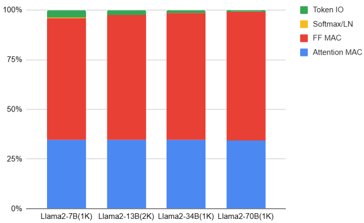
- Attention 計算量的比例大約是 1/3 (33%), MLP 計算量比例大約是 2/3 (66%).
計算量
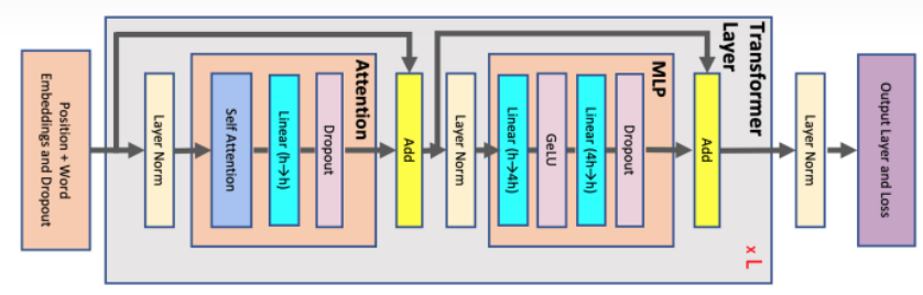
Training/Inference
Self attention
b = batch 在 training 時,會有 batch input, 在 inference 是 batch = 1 for ChatGPT model.
s = n_ctx (input tokens)
h = d_model ( = num_head * d_head)
- 此處考慮 batch size, 因爲 training.
- ChatGPT inference 的 batch size = 1. 以及在某些 network (大小網絡) batch size > 1 可以加速。
K, Q, V: Mapping Matrix : $Q = x_{in} W_Q,K = x_{in} W_K, V = x_{in} W_V$
- 計算 Q, K, V: input 和 output shape [b, s, h] x [h, h] –> [b, s, h]
- 計算量 $3 * 2 b s h^2 = 6 b s h^2$
QK: Attention matrix $x_{out} = \text{softmax}\left( \frac{Q K^T}{\sqrt{h}}\right) \cdot V \cdot W_O + x_{in}$
- 此處要考慮 multi-heads, 因此把 3D 的 Q, K, V [b, s, h] reshape 成 4D [b, head_num, s, per_head_hidden_size] where h = d_model = head_num * per_head_hidden_size
- $Q K^T$ 矩陣的 input 和 output [b, head_num, s, per_head_hidden_size] x [b, head_num, per_head_hidden_size, s] –> [b, head_num, s, s]
- 計算量: $2 b s^2 h$! 注意如果是 long context, s 可能會非常大, 1/2K -> 4/8/16/32K
Softmax $x_{out} = \text{softmax}\left( \frac{Q K^T}{\sqrt{h}}\right) \cdot V \cdot W_O + x_{in}$
- input 和 output shape 都是: [b, head_num, s, s]
- Softmax 計算量: $2 s^2 \text{head}_{num}$! 注意如果是 long context, s 可能會非常大, 1/2K -> 4/8/16/32K
Score $x_{out} = \text{softmax}\left( \frac{Q K^T}{\sqrt{h}}\right) \cdot V \cdot W_O + x_{in}$
- input 和 output shape 都是: [b, head_num, s, s] x [b, head_num, s, per_head_hidden_size] –> [b, head_num, s, per_head_hidden_size]
- 計算量: $2 b s^2 h$! 注意如果是 long context, s 可能會非常大, 1/2K -> 4/8/16/32K
Output Mapping $x_{out} = \text{softmax}\left( \frac{Q K^T}{\sqrt{h}}\right) \cdot V \cdot W_O + x_{in}$
- input 和 output shape 都是: [b, s, h] x [h, h] –> [b, s, h]
- 計算量: $2 b s h^2$
Self-Attention 的計算量
MAC: $6 b s h^2 + 2 b s^2 h + 2 b s^2 h + 2 b s h^2 = 8 b s h^2 + 4 b s^2 h$
Softmax: $2 s^2 \text{head}_{num}$
MLP
\[x_{mlp} = f_{gelu} (x_{out} W_1) W_2 + x_{out}\]- 第一個 FC (W1),矩陣乘法的輸入和輸出 [b, s, h] x [h, 4h] –> [b, s, 4h]
- 計算量是 $8 b s h^2$
- 第二個 FC (W2),矩陣乘法的輸入和輸出 [b, s, 4h] x [4h, h] –> [b, s, h]
- 計算量是 $8 b s h^2$
MLP 的計算量
MAC: $16 b s h^2 $
Layer Normalization - 參數 $\gamma, \beta$ : $4 d_{model} = 4h$
- Self-attention 和 FFN 各有一個 layer normalization. 包含兩個可訓練的參數:縮放參數 $\gamma$ 和平移參數 $\beta$, 形狀都是 $d_{model}$. 因此兩個 layer normalization 的參數量是 $4 d_{model}$
- Input, output [b, s, h] –> [b, h]
- 計算量是 $4 bsh$
Self-attention + MLP 計算量
每個 transformer 層的計算量: $24 b s h^2 + 4 b s^2 h$
所以所有的計算量 = $l * (24 b s h^2 + 4 b s^2 h)$
還有一個計算量的大頭是 input 和 output token to 字
- Input, output [b, s, h] x [h, V] –> [b, s, V]
- 計算量 2 b s h V.
- Total : $2 b s h V + l * (24 b s h^2 + 4 b s^2 h)$
參數量和計算量的關係
Short context ( $s \ll h$): 假設当隐藏维度 h 比较大,且远大于序列长度 s 时, 我们可以忽略一次项,计算量可以近似为
計算量 ~ $24 l b s h^2$, 此時對應的參數量是 $12 l h^2$ (和 s 無關!),一次得到 $b s$ tokens.
-
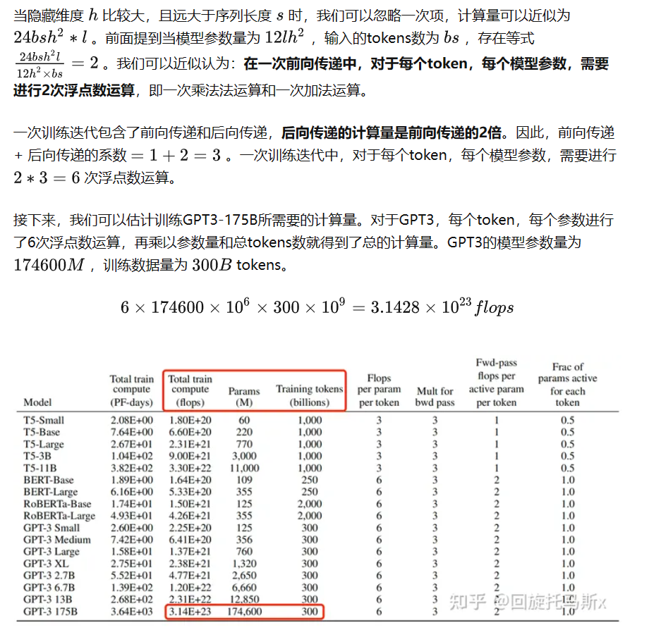
總計算量 : ~ 2 x 參數量 x 輸入 tokens! 可以近似認爲: 在一次前向传递中,对于每个token,每个模型参数,需要进行2次浮点数运算,即一次乘法法运算和一次加法运算。
-
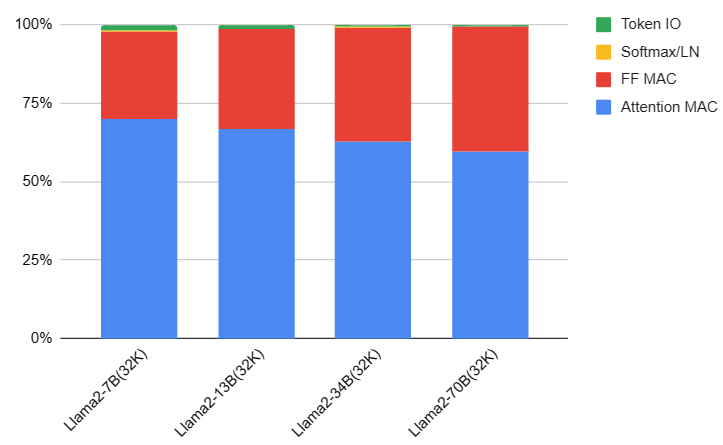
下圖可以看出 Llama2 1/2/4K context 的計算量/token 大約是參數量 x 2. 但是在 32K long context 的 attention 計算 ($4bs^2 h$) 量大幅增加。
-
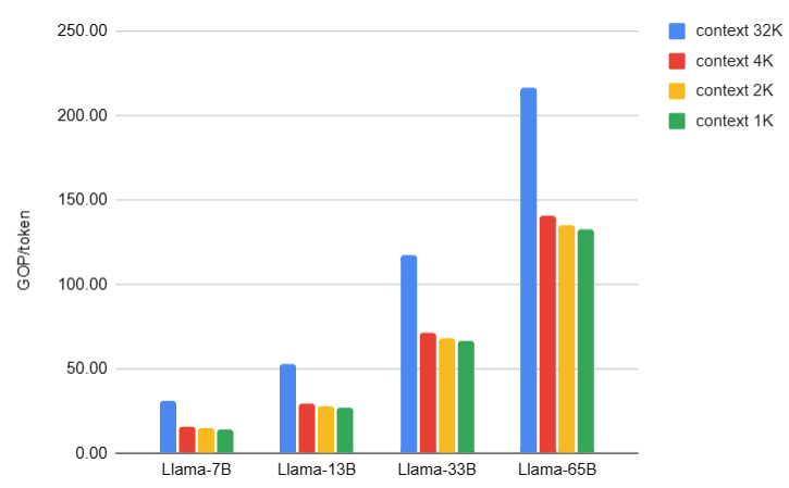
- 另外在 attention 計算量的比例大約是 1/3 (33%), MLP 計算量比例大約是 2/3 (66%).
-
下圖是 Llama2 with short context (1K) 的計算量比例:
-
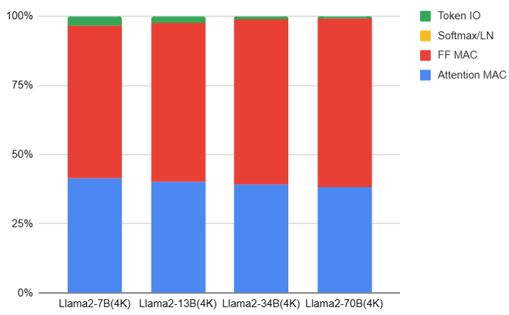
下圖是 Llama2 with default context (4K) 的計算量比例:(attention 計算量比例增加 from 34% to 40%)
-
下圖是 Llama2 with super long context (32K) 的計算量比例:(attention 計算量比例增加到 60-70%)
-
- 一次训练迭代包含了前向传递和后向传递,后向传递的计算量是前向传递的2倍。因此,前向传递 + 后向传递的系数 =1+2=3 。一次训练迭代中,对于每个token,每个模型参数,需要进行 2∗3=6 次浮点数运算。
Example: LLama-7B Inference
如果是 inference: bs = 1 per token.
如果是 training: bs 非常大
A: input token and first output token: 1024 output at 1 sec = 2 x 參數量 (7B=7G parameter) x 1024 = 14 TOPs
B: sustained output tokens: 2 x 參數量 (7B model = 7G parameter) x output token rate = 14 GOP/token x 10 token/sec = 140 GOP/sec
Example: GPT3-175B Training
每个token,每个参数进行了6次浮点数运算,再乘以参数量和总tokens数就得到了总的计算量。GPT3的模型参数量为 175B ,训练数据量为 300B tokens。
Training 計算量: 6 x 175B x 300B = 3.15 x 10^23 Flop
3.2 训练时间估计 (Training)
模型参数量和训练总tokens数决定了训练transformer模型需要的计算量。给定硬件GPU类型的情况下,可以估计所需要的训练时间。给定计算量,训练时间(也就是GPU算完这么多flops的计算时间)不仅跟GPU类型有关,还与GPU利用率有关。计算端到端训练的GPU利用率时,不仅要考虑前向传递和后向传递的计算时间,还要考虑CPU加载数据、优化器更新、多卡通信和记录日志的时间。一般来讲,GPU利用率一般在 0.3∼0.55 之间**。
上文讲到一次前向传递中,对于每个token,每个模型参数,进行2次浮点数计算。使用激活重计算技术来减少中间激活显存(下文会详细介绍)需要进行一次额外的前向传递,因此前向传递 + 后向传递 + 激活重计算的系数=1+2+1=4。使用激活重计算的一次训练迭代中,对于每个token,每个模型参数,需要进行 2∗4=8 次浮点数运算。在给定训练tokens数、硬件环境配置的情况下,训练transformer模型的计算时间为: