[@hosniTopImportant2023]
Source
Prompt Cache: Modular Attention Reuse For Low-Latency Inference
https://arxiv.org/pdf/2311.04934.pdf
[@gimPromptCache2023]
LLM
LLM 使用情境
基本上 LLM 有很明顯的兩種使用模式:
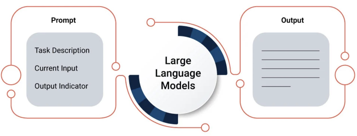
- Prompt 模式:就是輸入文本,可以很長,例如一篇文章。或是很短,只是命令或對話。
- Generation 模式:即是輸出文本,同樣可以很長,例如生出一篇文章。或是很短,例如摘要或對話。
- 什麽是影響 LLM 的體驗?
- 如何比較不同 LLM 實現的性能?A 公司/方法的 Llama2 和 B 公司/方法的 Llama2 的性能比較
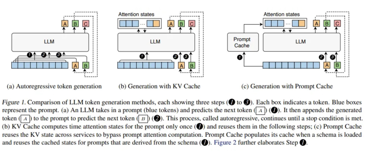
先看 LLM 最原汁原味的 autoregressive generation. 就是下圖左 (a). [@gimPromptCache2023]。
Autoregressive Generation
幾個特點:
- 只有一種 generative mode:假設 prompt 有 k 個 tokens. 第一次產生一個 token A. 下一次的 input 就是 k+1 個 token (包含 token A), 產生 token B. 再下一次的 input 就是 k+2 tokens (包含 A and B).
- 因為沒有 (KV) Cache, 每次的 input token 都會加一,越來越大。每次 generate one output token 都需要重新計算所有 input token 的 attention vectors. 好處是只需要載入 LLM 參數,而不需要載入 cache. 可以說是用計算換頻寬。缺點是產生 output token 的 latency 不只是 BW bound, 也是 computation bound. 另外 power 會增加。
KV Cache Generation
基本概念和前面方法一樣。但是引入 KV cache 儲存之前計算過的每個 token 的 attention vectors. 如上圖 (b)
幾個特點:
- 引入 KV cache 可以不用重新計算 attention vectors of previous computed tokens. 因此每次產生新的 output token 需要重新載入 LLM 參數和 KV cache, 但是大幅減少計算量。所以是頻寬 limited.
- 每次需要重新更新 KV cache. 如果 KV cache 滿了,就會移除最早的 entry.
Prompt Cache Generation
[@gimPromptCache2023] 的文章是假設一些固定的 prompt 模型,稱為 schema. 可以預先計算所謂的 “prompt cache”. 避免之後需要一再重複計算 (這不就是 KV Cache 的功能?)。
Prompt cache 和 KV cache 有什麼不同?
- Prompt cache 其實是 KV cache 的延伸。對於固定的 prompt template, 稱為 schema, 可以預先計算 attention vectors。
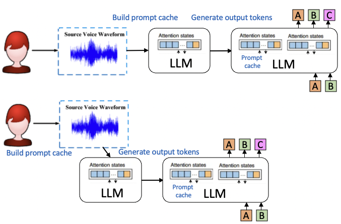
Prompt cache 可以用於 sequential prompt input, 特別是比較慢的語音或是鍵盤輸入。
- Pipeline prompt cache 的建立,建立 prompt cache 的時間藏在鍵盤輸入或語音輸入辨識中。
- 如果輸入的是一大篇文章,遠快於 prompt cache 建立的速度,當然就無法把建立 prompt cache 的時間藏住。就和 KV cache 的做法一樣。
- LLM 提供額外的好處就是 error correction. 一般 LLM 的能力足以 correct 語音中的冗余和鍵盤輸入的 typo.
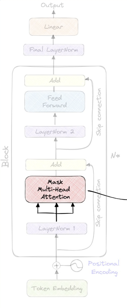
- 更重要的是 prompt cache 的建立可以是 chunk-by-chunk, 不必一部到位。因為計算每個 token 的 attention vectors 是先 apply 一個 “causal mask”!
- Prompt cache 的最大好處是縮短 first token latency. (1) 如果是 paper 的預先計算 attention vectors, 可以節省時間和計算;(2) 如果是以上 pipeline prompt cache 可以把建立 prompt cache 的時間藏在鍵盤輸入或語音辨識中。
LLM 的體驗
-
Prompt 處理完產生第一個 output token latency, 就是產生上上圖的 token A 的 latency. 或是 prompt 的處理速度。
-
後續 output token B, C, … ,也就是 output token 生成的速度。
-
也可以結合 1 and 2, 定義端到端的 latency. 不過速度和 token 數目無關,但是 latency 和 input/output token 數目直接正比。所以需要定義 input/output token 數目。
- 常見的方法:(input token, output token) = (1024, 10) 這比較適合語音產生第一句話的時間。
- 或是 (input token, output token) = (512, 512) 比較適合文本的輸入和輸出。
對應 LLM 1 and 2 包含兩個部分: prompt phase 和 generation phase.
- Prompt phase 就是 LLM 處理 input token, 計算 (causal) attention vector of each token and store in prompt KV cache (for KV cache 和 prompt cache) 的過程。
- Generation phase 則是接下來生成 output token, 並且 update KV cache 的過程。
LLM 重要 KPI
Generation phase (sequentially generate output tokens)
-
Average memory bandwidth per token (GB/sec): 產生一個 output token 所需要的 memory bandwidth. 一般包含兩個部分
- Static (read) memory BW: 產生每個 output token 都需要讀入 LLM weight (W) 參數。
- Static memory BW = Model size x precision
- 例如 INT8 of 7B LLM, 1byte x 7B = 7GB, 如果是 FP16, 2byte x 7B = 14 GB. 如果是 INT4 (W4) of 7B LLM, 0.5 byte x 7B = 3.5GB.
- Dynamic (read/write) memory BW: 主要是讀入和寫出 KV cache. 基本和 $n_{ctx}$ 和 precision 成正比。
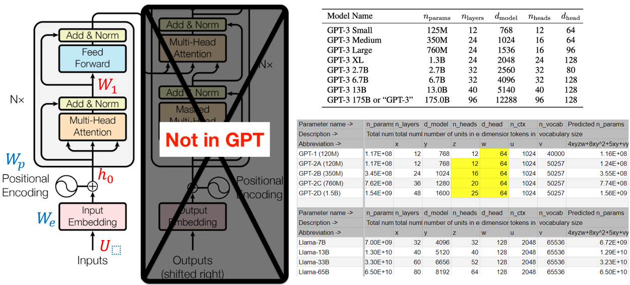
- KV cache = 2 (for K/V) x $n_{ctx}$ x precision x $d_{model}$ x $n_{layer}$.
- 例如 2K context, INT8 activation (A8). KV cache 2 x 2048 x 1 x 4096 x 32 = 0.54GB.
- Dynamic memory 至少要讀一次。可能要寫出一次,如果是用 ring buffer, 只需要部分寫出。
- Static + dynamic memory BW 最理想狀況: 3.5GB + 0.54GB ~ 4GB/token for W4A8 7B model.
- Static (read) memory BW: 產生每個 output token 都需要讀入 LLM weight (W) 參數。
-
Average output token rate (token/sec): 每次產生一個 output token, 都需要從 DRAM 重新 load LLM 參數和 KV cache。所以是 memory bandwidth limit.
-
Total memory BW = output token rate x BW per token x peak-to-average ratio
-
如果 (64-bit DDR5 6400MHz) memory BW = 50GB/sec, peak-to-average BW ratio = 1.25, 4GB/token
可以得到最佳的 output token rate = 50GB/sec / 1.25 / 4GB/token = 10 token/sec
-
Prompt phase (processing input tokens in parallel)
- Prompt processing rate (token/sec): 因為 input prompt 可以被同時平行處理 (上上圖的藍色 input tokens)。這和 generation phase 完全是 BW limit 不相同。如果一次處理 128 tokens, 則 memory BW 的效率就提高 128 倍。
- BW limit 的 prompt processing rate = 128 x output token rate = 1280 token/sec,顯然 prompt processing 不一定是 limiting factor.
- Computation limit 的 prompt processing rate. 每個 input token 所需要的算力基本包含
- Static processing: 2 x model size x precision = 2 x 7G x 1 = 14 GOPS
- Dynamic processing: 2 x KV cache x precision = 2 x 0.5G x 1 = 1 GOPS
- Static + dynamic processing 需要 14 + 1 = 15 GOPS/token. 注意這是在 KV cache 建立才需要加上 dynamic processing 算力。
- 在 KV cache 建立後,generation phase 需要的算力如上。比起 BW limit 的 latency 小的多。
- 如果不用 KV cache, 而是直接 autoregressive, 需要算力就是 k x 14 GOPS! k 每次都會加 1, 最後會是 computation dominant 而非 memory BW dominant.
- 所以 prompt mode rate = NPU TOPS/sec x utilization rate / TOPS/token
- 假設 NPU 40 TOPS/sec, urate = 25%, 15 GOPS/sec : 40 TOPS/sec x 25% / 15 GOPS/token = 667 tokens/sec limited by computation power
- 如果加上 memory BW limit (assuming 128 token processing): 1/(1/667+1/1280) = 440 token/sec
- 所以 first output token latency = context length / prompt mode rate
- 假設 context length = 1024 tokens, first token latency = 1024 / 667 = 1.5 sec
End-to-end latency
一旦有 prompt processing rate 和 output generation rate. 很容易可以計算
end-to-end latency of (Input token, output token) = input token / prompt rate + output token / generation rate
- (1024, 10) = 1024 / 440 token/sec + 10 / 10 token/sec = 2.3 sec + 1 sec = 3.3 sec. for 語音。
- (512, 512) = 512 / 440 + 512 / 10 = 52.3 sec. for 文章。
- 很明顯兩者都無法接受。改善方法
- 提高 memory BW 可以提升 generation rate, 減少 generation latency.
- 提高 NPU 算力可以提升 prompt rate, 減少 prompt latency.
[@hosniTopImportant2023]
Reference
Gim, In, Guojun Chen, Seung-seob Lee, Nikhil Sarda, Anurag Khandelwal,
and Lin Zhong. 2023. “Prompt Cache: Modular Attention Reuse for
Low-Latency Inference.” November 7, 2023.
http://arxiv.org/abs/2311.04934.
Hosni, Youssef. 2023. “Top Important LLM Papers for the Week from 06/11
to 12/11.” Medium. November 15, 2023.
https://pub.towardsai.net/top-important-llm-papers-for-the-week-from-06-11-to-12-11-f9968bd8edbf.