大(語言)模型參數微調 PEFT

Source

Moral -> Guilty -> Emotion

Parameter-Efficient Fine-Tuning for Large Models: A Comprehensive Survey https://arxiv.org/abs/2403.14608

Towards a Unified View of Parameter-Efficient Transfer Learning https://arxiv.org/abs/2110.04366

LLMs from scratch - very good and well written example

煉丹五部曲

1. 應用 (起死回生，長生不老，美顔)：analytic (spam, sentiment) or generative (summarization)

2. 靈材：datasets, tokenizer, embedding

3. 丹方：model

4. 丹爐：Nvidia GPU (和財力有關)

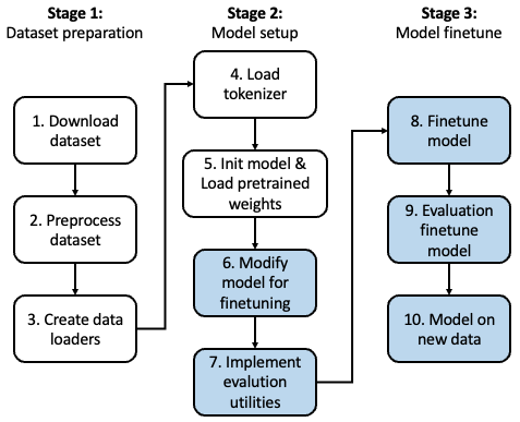
5. 煉製：training: data_loader, loss function, optimizer
   1. Fine-tune pre-trained model
6. 評估：evaluation: accuracy, BLEU

我們現在討論 step 4.1, Finetune pre-trained model!

微调：大型语言模型通常在下游任务上进行微调，方法是在预训练模型的顶部添加特定任务的层。这个微调过程调整了嵌入和其他模型参数，以提高目标任务的性能。

Why (Full parameter) Fine-Tuning or Parameter Efficient Fine-Tuning

Training from scratch 需要 (1) 大量的 data (Giga words, Tera words, …), D; (2) 大量的 resources (算力，內存，和時間) ~ D (Data) x W (model size).

如果是算力 bound, D x W ~ 算力 x 時間。如果是內存頻寬 bound ~ 內存頻寬 x 時間。大多情況是算力和內存頻寬兩者都有影響。

Full (parameter) fine-tune pre-trained model 在 training 最大的好處是: 不需要大量的 data, 只需要少量的 data (Kiko words or Mega words?)，i.e. (D -> 小 D). 所以另一個附加的好處是不需要大量的算力。但仍然需要同樣的內存以及內存頻寬 for model storage and access. 對於 inference 完全沒有沒有影響。

而 Parameter Efficient FT 只調整部分的參數 (W -> 小 W，一般是幾 %)。對於 training, 節省更多的算力和内存頻寬。但是對於 inference 則不一定。在某些情況可能完全沒有影響 (e.g. selective parameter fine tuning, LoRA merge the parameter)，也有可能多出算力。(e.g. adaptor, LoRA of parallel computation)

	from scratch	Full fine tuning	Adaptor	Selective	LoRA	Soft Prefix
Training	$D \times W$	$\Delta D \times W$	$\Delta D \times \Delta W$	$\Delta D \times \Delta W$	$\Delta D \times \Delta W$	$\Delta D \times \Delta W?$
Inference	$W$	$W$	$W + \Delta W$	$W$	$W$ or $W+\Delta W$	$W \times 1.0?$

• D 是完整的 data, W 是 model weight.

• software prefix 的 context length 會變長，所以 inference computation 會變多。

一般對於 from scratch vs. full fine tuning 的討論沒有問題。因爲差異很大。對於 full fine tune vs. PEFT 則有不同的意見。有一部分人認爲 full fine tuning 所花的時間和 PEFT 沒有差太多，而且只是 one-time. 反而 inference 時要多計算。因爲 inference 發生的頻率遠高於 training, 所以傾向 full fine tuning. 不過對於 edge fine tune，PEFT, 特別是 LoRA 還是可以節省大量算力。另外 LoRA 還可以 enable multiple applications. 因此 PEFT 還是顯學！

PEFT 的分類

先說 baseline: Full Fine Tuning, 或是 full tuning. 即是在 pre-tune network 的基礎上，可以調整所有的參數，但是不改變 network topology.

PEFT (parameter efficient fine tuning): 只調整（或是加入）部分的參數 for downstream work.

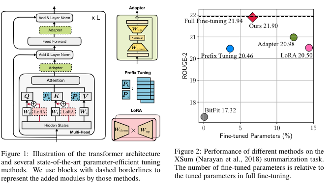
• Adaptor: physical layer 插入原來的網路。會改變原來的 network topology，以及加入新的參數，所以效果最好？
• Software prefix: 在 prompt 直接加上 finetune parameter。不會改變原來的網路和參數，所以效果最小？
• LoRA: 只是改變部分參數，不會改變 network topology. 所有效果介於之間？

LoRA Fine-Tune

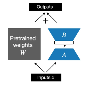
LoRA 使用兩個 Low Rank matrix, A and B, 作爲 fine tune parameters.

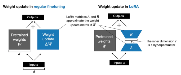
• 在 training 或是 full fine-tuning, 或是更準確 back-prop phase: $W_{updated} = W + \Delta W$.
• 在 PEFT 的 LoRA 中，$W$ is frozen, $\Delta W \approx A B$. $W_{updated} = W + A B$. $A, B$ 的初始值為 0, 而不至於影響原來的結果。
• 在 inference phase, 或是 forward phase, $x(W+\Delta W) = x(W+AB)$. 有兩種計算方法，一個是把 $AB$ 合入 $W$, 好處是不會有額外的計算。另一種方法是分開計算最後整合。 $x(W+\Delta W) = xW+xAB$​. 壞處是額外的計算和内存以及内存頻寬。好處是保留原來的 base model. 所以可以有多個 LoRA 切換。
• LoRA 可以調整的部分一般包含：feedforward layer, output layer, 以及 attention block 中的 K, Q, (and V?) mapping layers.

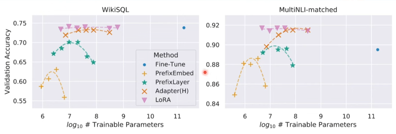
以下是不同的 PEFT 在 LLM 的結果。LoRA 的效果最好，接近或超過 full fine tune。而且對 trainable parameter size 很 robust.

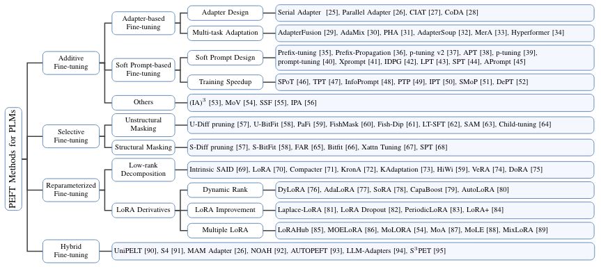
更細的分類：

1. Adaptor: serial, parallel, hybrid.
2. LoRA (reparameter): LoRA, DoRA, DyLoRA
3. 加一個子類：selective fine tuning

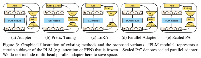
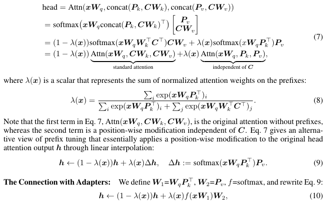
PEFT 的 Unified View

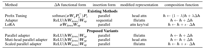
PEFT 的實例 :

我們使用 GPT2-small model 作為 PEFT 例子。

GPT2 原始的 model size: emb_dim: 768, n_layers: 12, n_heads: 12. 總參數量：124M (可以參考 LLM parameter excel file).

LLM 直接用 Text Classification

LLM 可以不需要 retrain 或是 fine-tune 直接回答一個訊息是否為 spam，稱為 0-shot. 也可以直接在 prompt 提供 k 個例子，稱為 k-shots. 不過這種無需 retrain/fine-tune 方式和 LLM 本身的能力有關，基本上 LLM 需要比較大的模型 (7B or above) 經過適當 data 的訓練才有比較好的結果。以 GPT2 (124M) 為例，結果並不令人滿意。

Fine-tune 則是一個非常好的方法讓小型 LLM 處理特定領域任務 (domain specific task)

1 2 3 4 5 6 7 8 9 10 11 12 13 14 15

text = ( "Is the following text 'spam'? Answer with 'yes' or 'no':" " 'You are a winner you have been specially" " selected to receive $1000 cash or a $2000 award.'" " Answer with 'yes' or 'no'." ) token_ids = generate_text_simple( model=model, idx=text_to_token_ids(text, tokenizer), max_new_tokens=23, context_size=BASE_CONFIG["context_length"] ) print(token_ids_to_text(token_ids, tokenizer))

1	Is the following text 'spam'? Answer with 'yes' or 'no': 'You are a winner you have been specially selected to receive $1000 cash or a $2000 award.' Answer with 'yes' or 'no'. Answer with 'yes' or 'no'. Answer with 'yes' or 'no'. Answer with 'yes'

修改 LLM for 文本分類

在開始微調之前，我們先對 LLM 做個小手術。把原來文本輸出 ‘yes, this is a SPAM’, 變成 binary output, 0: negative, 1: positive.

小手術包含兩個 dimensions: (1) embedding (spatial) dimension, 50257 vocab 變成 2 binary; (2) token context (temporal) dimension, 取出第一個 (或是最後一個) token?

修改 embedding (spatial) dimension

不過第一步是修改最後 output layer (linear, no softmax?) 從 $768 \to50257$ 變成 $768\to2$​，如下圖。

Q: no softmax at the output?

A: No, model 的 output 是 logits. 在 training 時，會用 cross-entropy loss function 作 back-prop. Cross-entropy 本身就類似 softmax function. 在 inference 時，只要 sample 最大值，也不需要 softmax. Softmax output 一般是要提供分類機率值，常用於 computer vision. LLM 似乎非常少用 softmax as output。

1 2	num_classes = 2 model.out_head = torch.nn.Linear(in_features=768, out_features=num_classes)

修改 token context (temporal) dimension

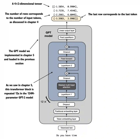
修改 embedding layer model 後的 input 和 output:

• Input tensor shape: (batch_size=1, input_num_tokens). [1,4] in the following case.
• Output tensor shape: (batch_size=1, output_num_tokens, num_classes=2). [1, 4, 2] in the following case. 為什麼 output token number 剛好也等於 4? 巧合嗎？

1 2 3 4 5 6 7 8 9 10 11 12 13 14 15 16 17 18 19 20

inputs = tokenizer.encode("Do you have time") inputs = torch.tensor(inputs).unsqueeze(0) print("Inputs:", inputs) print("Inputs dimensions:", inputs.shape) # shape: (batch_size, num_tokens) --------------- output ----------------- Inputs: tensor([[5211, 345, 423, 640]]) Inputs dimensions: torch.Size([1, 4]) ----------------------------------------- outputs = model(inputs) print("Outputs:\n", outputs) print("Outputs dimensions:", outputs.shape) # shape: (batch_size, num_tokens, num_classes) --------------- output ----------------- Outputs: tensor([[[-1.5854, 0.9904], [-3.7235, 7.4548], [-2.2661, 6.6049], [-3.5983, 3.9902]]]) Outputs dimensions: torch.Size([1, 4, 2]) ------------------------------------------

因此我們取出最後一個 token 作為最後的 output，也就是 outputs[:, -1, :] = [-3.5983, 3.9902] 。

1	print("Last output token:", outputs[:, -1, :])

我們定義微調的 loss function (這和 LLM training 的 loss function 不同)。

重要和微妙：model output, i.e. logits 是用 one-hot format (01, 10) 代表 2 classes. 但是 target_batch 中的 label 卻是 binary format (0: spam negative; 1: spam positive). 理論上計算 loss function，需要把 target_batch 的 binary format 轉換成 one-hot format. 不過 torch 的 cross-entropy loss 會自動處理這個轉換。對 binary classes 或是 multiple classes 分類看起來比較簡潔。

1 2 3 4 5

def calc_loss_batch(input_batch, target_batch, model, device): input_batch, target_batch = input_batch.to(device), target_batch.to(device) logits = model(input_batch)[:, -1, :] # Logits of last ouput token loss = torch.nn.functional.cross_entropy(logits, target_batch) return loss

我們同樣定義 accuracy function by sampling the maximum output. 如前所述，我們不用 softmax 計算機率。只用 argmax 取最大值。

1 2 3 4 5 6 7 8 9 10 11 12 13 14 15 16

@torch.no_grad() # Disable gradient tracking for efficiency def calc_accuracy_loader(data_loader, model, device, num_batches=None): model.eval() correct_predictions, num_examples = 0, 0 for i, (input_batch, target_batch) in enumerate(data_loader): if i < num_batches: input_batch, target_batch = input_batch.to(device), target_batch.to(device) logits = model(input_batch)[:, -1, :] # Logits of last ouput token predicted_labels = torch.argmax(logits, dim=-1) num_examples += predicted_labels.shape[0] correct_predictions += (predicted_labels == target_batch).sum().item() else: break return correct_predictions / num_examples

沒有微調的分類結果應該接近盲猜，也就是 50%.

1 2 3 4 5 6 7 8 9 10 11 12

torch.manual_seed(123) train_accuracy = calc_accuracy_loader(train_loader, model, device, num_batches=10) val_accuracy = calc_accuracy_loader(val_loader, model, device, num_batches=10) test_accuracy = calc_accuracy_loader(test_loader, model, device, num_batches=10) print(f"Training accuracy: {train_accuracy*100:.2f}%") print(f"Validation accuracy: {val_accuracy*100:.2f}%") print(f"Test accuracy: {test_accuracy*100:.2f}%") --------------- output ----------------- Training accuracy: 46.25% Validation accuracy: 45.00% Test accuracy: 48.75%

接下來就是 PTFE, 也就是微調。

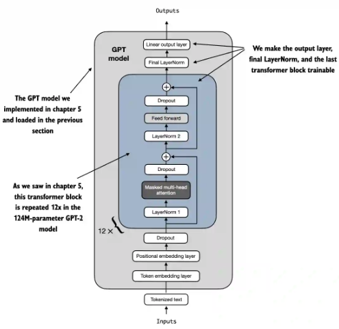
Selective fine-tuning

最簡單的 selective fine-tune 就是 fine tune 最後的 output layer(s)。其實這是早期 ML 的 transfer learning。

不過把最後的 transformer layer h[11], 和對應的 LayerNorm layer 一起 Fine tune, 效果更好。

1 2 3 4 5 6 7 8 9 10 11 12 13 14 15 16 17 18 19 20 21 22 23

# Freeze 所有的 model 參數 for param in model.parameters(): param.requires_grad = False # Set the last transformer block to trainable for param in model.transformer.h[11].parameters(): # Accessing the last transformer block (index 11) param.requires_grad = True # Access the LayerNorm module connecting the last transformer block to the output layer layer_norm_module = model.transformer.ln_f # Set the LayerNorm module to trainable for param in layer_norm_module.parameters(): param.requires_grad = True # Set the output head (final linear layer) to trainable for param in model.lm_head.parameters(): param.requires_grad = True total_params = sum(p.numel() for p in model.parameters() if p.requires_grad) print(f"Total trainable parameters: {total_params:,}") --------------- output ----------------- Total trainable parameters: 7,090,946

• 可調的參數：7.1M, 比起 142M, 約為 5.7%.
• Fine-tune 之後的 test accuracy ~ 90%.

1 2 3 4 5 6 7 8 9 10 11

train_accuracy = calc_accuracy_loader(train_loader, model, device) val_accuracy = calc_accuracy_loader(val_loader, model, device) test_accuracy = calc_accuracy_loader(test_loader, model, device) print(f"Training accuracy: {train_accuracy*100:.2f}%") print(f"Validation accuracy: {val_accuracy*100:.2f}%") print(f"Test accuracy: {test_accuracy*100:.2f}%") --------------- output ----------------- Training accuracy: 91.44% Validation accuracy: 93.29% Test accuracy: 90.33%

LoRA

如前所述，LoRA 是用 AB low rank matrix 做微調。

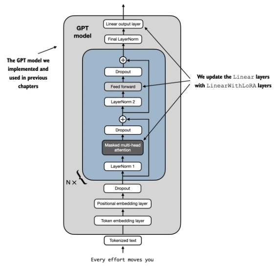
我們對使用 LoRALayer 取代原來的 Linear Layer: transformer 中的 Feed forward, attention block 的 K,Q,(and V?), 以及 output layer.

以下是需要修改的 code.

1 2 3 4 5 6 7 8 9 10 11 12 13 14 15 16 17 18 19 20 21 22 23

class LoRALayer(torch.nn.Module): def __init__(self, in_dim, out_dim, rank, alpha): super().__init__() std_dev = 1 / torch.sqrt(torch.tensor(rank).float()) self.A = torch.nn.Parameter(torch.randn(in_dim, rank) * std_dev) self.B = torch.nn.Parameter(torch.zeros(rank, out_dim)) self.alpha = alpha def forward(self, x): x = self.alpha * (x @ self.A @ self.B) return x class LinearWithLoRA(torch.nn.Module): def __init__(self, linear, rank, alpha): super().__init__() self.linear = linear self.lora = LoRALayer( linear.in_features, linear.out_features, rank, alpha ) def forward(self, x): return self.linear(x) + self.lora(x)

原始的 GPT2 model 是 124M.

1 2 3 4

total_params = sum(p.numel() for p in model.parameters() if p.requires_grad) print(f"Total trainable parameters before: {total_params:,}") Total trainable parameters before: 124,441,346

LoRA 的 trainable parameter: 1.3M. 比例只有 1%!.

1 2 3 4 5 6

replace_linear_with_lora(model, rank=8, alpha=8) total_params = sum(p.numel() for p in model.parameters() if p.requires_grad) print(f"Total trainable LoRA parameters: {total_params:,}") Total trainable LoRA parameters: 1,333,264

LoRA 的 accuracy ~ 98% 看起來還不錯！

1 2 3 4 5 6 7 8 9 10 11 12 13

from previous_chapters import calc_accuracy_loader train_accuracy = calc_accuracy_loader(train_loader, model, device) val_accuracy = calc_accuracy_loader(val_loader, model, device) test_accuracy = calc_accuracy_loader(test_loader, model, device) print(f"Training accuracy: {train_accuracy*100:.2f}%") print(f"Validation accuracy: {val_accuracy*100:.2f}%") print(f"Test accuracy: {test_accuracy*100:.2f}%") --------------- output ----------------- Training accuracy: 100.00% Validation accuracy: 96.64% Test accuracy: 98.00%