大(語言)模型參數微調 PEFT

Source

Moral -> Guilty -> Emotion

Parameter-Efficient Fine-Tuning for Large Models: A Comprehensive Survey https://arxiv.org/abs/2403.14608

Towards a Unified View of Parameter-Efficient Transfer Learning https://arxiv.org/abs/2110.04366

LLMs from scratch - very good and well written example (Chinese) https://mbd.baidu.com/newspage/data/landingsuper?rs=1120356222&ruk=xed99He2cfyczAP3Jws7PQ&urlext=%7B%22cuid%22%3A%22082Wa_ih2ilai2iK_u-LuliAvtYpa2a0gaSVfl8PviKo0qqSB%22%7D&isBdboxFrom=1&pageType=1&sid_for_share=&context=%7B%22nid%22%3A%22news_9255209899271066135%22,%22sourceFrom%22%3A%22bjh%22%7D

(English) https://magazine.sebastianraschka.com/p/building-a-gpt-style-llm-classifier

煉丹五部曲

1. 應用 (起死回生，長生不老，美顔)：analytic (spam, sentiment) or generative (summarization)

2. 靈材：datasets, tokenizer, embedding

3. 丹方：model

4. 丹爐：Nvidia GPU (和財力有關)

5. 煉製：training: data_loader, loss function, optimizer 4.1 Fine-tune pre-trained model

6. 評估：evaluation: accuracy, BLEU

我們現在討論 step 4.1, Finetune pre-trained model!

**微调：大型语言模型通常在下游任务上进行微调，方法是在预训练模型的顶部添加特定任务的层。这个微调过程调整了嵌入和其他模型参数，以提高目标任务的性能。

阅读完本文，你将找到以下 7 个问题的答案：

1. 需要训练所有层吗？
2. 为什么微调最后一个 token，而不是第一个 token？
3. BERT 与 GPT 在性能上有何比较？
4. 应该禁用因果掩码吗？
5. 扩大模型规模会有什么影响？
6. LoRA 可以带来什么改进？
7. Padding 还是不 Padding？

Why (Full parameter) Fine-Tuning or Parameter Efficient Fine-Tuning

Training from scratch 需要 (1) 大量的 data (Giga words, Tera words, …), D; (2) 大量的 resources (算力，內存，和時間) ~ D (Data) x W (model size).

如果是算力 bound, D x W ~ 算力 x 時間。如果是內存頻寬 bound ~ 內存頻寬 x 時間。大多情況是算力和內存頻寬兩者都有影響。

Full (parameter) fine-tune pre-trained model 在 training 最大的好處是: 不需要大量的 data, 只需要少量的 data (Kiko words or Mega words?)，i.e. (D -> 小 D). 所以另一個附加的好處是不需要大量的算力。但仍然需要同樣的內存以及內存頻寬 for model storage and access. 對於 inference 完全沒有沒有影響。

而 Parameter Efficient FT 只調整部分的參數 (W -> 小 W，一般是幾 %)。對於 training, 節省更多的算力和内存頻寬。但是對於 inference 則不一定。在某些情況可能完全沒有影響 (e.g. selective parameter fine tuning, LoRA merge the parameter)，也有可能多出算力。(e.g. adaptor, LoRA of parallel computation)

	Pre-train	Fully fine tuning (FFT)	Adaptor	Selective	LoRA	Soft Prefix
Training	$D \times W$	$\Delta D \times W$	$\Delta D \times \Delta W$	$\Delta D \times \Delta W$	$\Delta D \times \Delta W$	–
Inference	$B \times W$	$B \times W$	$B \times (W + \Delta W)$	$B \times W$	$B \times W$ or $B \times (W+\Delta W)$	$B \times W$

• D 是完整的 data, W 是 model weight.

• software prefix 的 context length 會變長，所以 inference computation 會變多。

一般對於 from scratch vs. full fine tuning 的討論沒有問題。因爲差異很大。對於 full fine tune vs. PEFT 則有不同的意見。有一部分人認爲 full fine tuning 所花的時間和 PEFT 沒有差太多，而且只是 one-time. 反而 inference 時要多計算。因爲 inference 發生的頻率遠高於 training, 所以傾向 full fine tuning. 不過對於 edge fine tune，PEFT, 特別是 LoRA 還是可以節省大量算力。另外 LoRA 還可以 enable multiple applications. 因此 PEFT 還是顯學！

	預訓練 (Pre-train)	持續預訓練	全微調 (FFT)	參數高效微調（PEFT）	檢索增強生成（RAG）	上下文學習 (ICL)
參數	100%	100%	100%	1-6%	–	–
數據	100%	10%	1%	1%	外部數據庫	幾個示例
GPU 小時	1000’s	100’s	10’s	1’s	1’s	0
方法	自監督學習*(SSL)	自監督學習(SSL)	監督學習（SL）或強化學習（RL）	監督學習（SL）	數據庫索引 （database indexing)	提示工程 (prompt engineering)
軟體	訓練	訓練	微調	微調	RAG + 推理	推理
目的	建立基礎模型	增強基礎模型	指令跟隨、人類對齊	自定義、風格變更	實時內容、減少幻覺	提高準確性

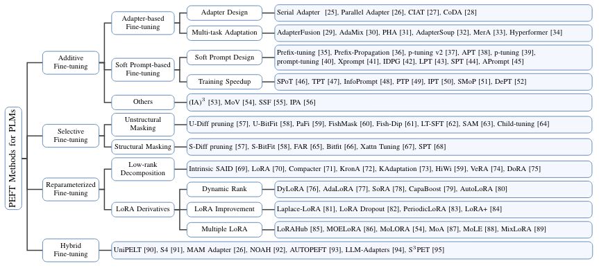
PEFT 的分類

先說 baseline: Full Fine Tuning, 或是 full tuning. 即是在 pre-tune network 的基礎上，可以調整所有的參數，但是不改變 network topology.

PEFT (parameter efficient fine tuning): 只調整（或是加入）部分的參數 for downstream work.

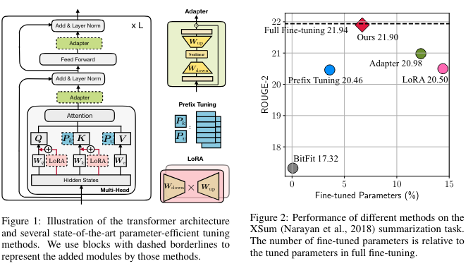
• Adaptor: physical layer 插入原來的網路。會改變原來的 network topology，以及加入新的參數，所以效果最好？
• Software prefix: 在 prompt 直接加上 finetune parameter。不會改變原來的網路和參數，所以效果最小？
• LoRA: 只是改變部分參數，不會改變 network topology. 所有效果介於之間？

LoRA Fine-Tune

LoRA 使用兩個 Low Rank matrix, A and B, 作爲 fine tune parameters.

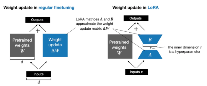
• 在 training 或是 full fine-tuning, 或是更準確 back-prop phase: $W_{updated} = W + \Delta W$.
• 在 PEFT 的 LoRA 中，$W$ is frozen, $\Delta W \approx A B$. $W_{updated} = W + A B$. $A, B$ 的初始值為 0, 而不至於影響原來的結果。
• 在 inference phase, 或是 forward phase, $x(W+\Delta W) = x(W+AB)$. 有兩種計算方法，一個是把 $AB$ 合入 $W$, 好處是不會有額外的計算。另一種方法是分開計算最後整合。 $x(W+\Delta W) = xW+xAB$​. 壞處是額外的計算和内存以及内存頻寬。好處是保留原來的 base model. 所以可以有多個 LoRA 切換。
• LoRA 可以調整的部分一般包含：feedforward layer, output layer, 以及 attention block 中的 K, Q, (and V?) mapping layers.

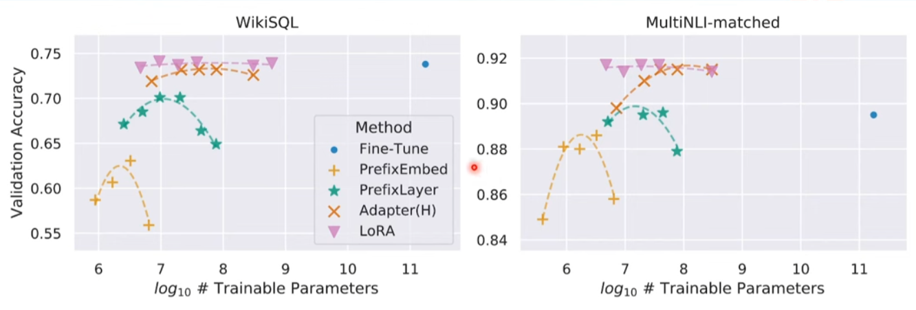
以下是不同的 PEFT 在 LLM 的結果。LoRA 的效果最好，接近或超過 full fine tune。而且對 trainable parameter size 很 robust.

更細的分類：

1. Adaptor: serial, parallel, hybrid.
2. LoRA (reparameter): LoRA, DoRA, DyLoRA
3. 加一個子類：selective fine tuning

PEFT 的 Unified View

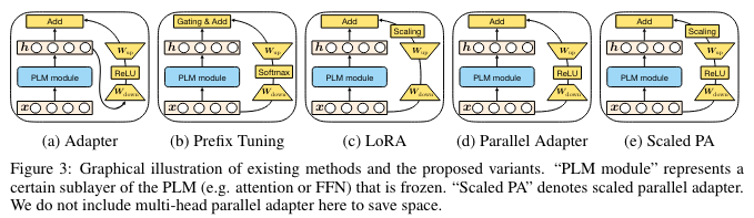
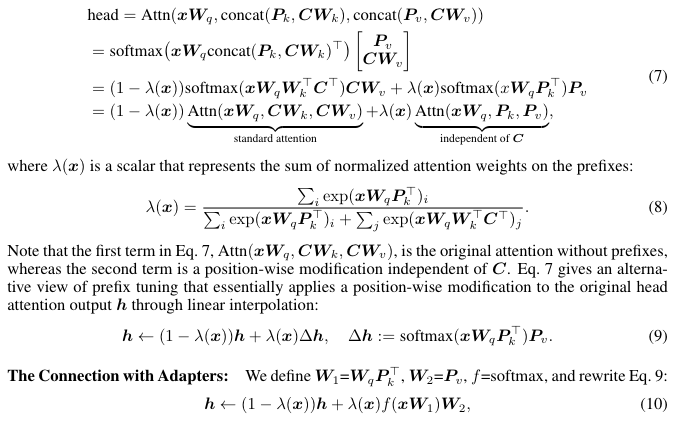
先看 attention 的公式: \(\begin{aligned} & \text { head }=\operatorname{Attn}\left(\boldsymbol{x} \boldsymbol{W}_q, \operatorname{concat}\left(\boldsymbol{P}_k, \boldsymbol{C} \boldsymbol{W}_k\right), \operatorname{concat}\left(\boldsymbol{P}_v, \boldsymbol{C} \boldsymbol{W}_v\right)\right) \\ & =\operatorname{softmax}\left(\boldsymbol{x} \boldsymbol{W}_q \operatorname{concat}\left(\boldsymbol{P}_k, \boldsymbol{C} \boldsymbol{W}_k\right)^{\top}\right)\left[\begin{array}{c} \boldsymbol{P}_v \\ \boldsymbol{C} \boldsymbol{W}_v \end{array}\right] \\ & =(1-\lambda(\boldsymbol{x})) \operatorname{softmax}\left(\boldsymbol{x} \boldsymbol{W}_q \boldsymbol{W}_k^{\top} \boldsymbol{C}^{\top}\right) \boldsymbol{C} \boldsymbol{W}_v+\lambda(\boldsymbol{x}) \operatorname{softmax}\left(x \boldsymbol{W}_q \boldsymbol{P}_k^{\top}\right) \boldsymbol{P}_v \\ & =(1-\lambda(\boldsymbol{x})) \underbrace{\operatorname{Attn}\left(\boldsymbol{x} \boldsymbol{W}_q, \boldsymbol{C} \boldsymbol{W}_k, \boldsymbol{C} \boldsymbol{W}_v\right)}_{\text {standard attention }}+\lambda(\boldsymbol{x}) \underbrace{\operatorname{Attn}\left(\boldsymbol{x} \boldsymbol{W}_q, \boldsymbol{P}_k, \boldsymbol{P}_v\right)}_{\text {independent of } \boldsymbol{C}} \text {, } \end{aligned}\)

where $\lambda(x)$ is a scalar that represents the sum of normalized attention weights on the prefixes:

\[\lambda(\boldsymbol{x})=\frac{\sum_i \exp \left(\boldsymbol{x} \boldsymbol{W}_q \boldsymbol{P}_k^{\top}\right)_i}{\sum_i \exp \left(\boldsymbol{x} \boldsymbol{W}_q \boldsymbol{P}_k^{\top}\right)_i+\sum_j \exp \left(\boldsymbol{x} \boldsymbol{W}_q \boldsymbol{W}_k^{\top} \boldsymbol{C}^{\top}\right)_j}\]

注意 attention 方程中的第一項 $\operatorname{Attn}\left(\boldsymbol{x} \boldsymbol{W}_q, \boldsymbol{C} \boldsymbol{W}_k, \boldsymbol{C} \boldsymbol{W}_v\right)$ 是沒有 prefixes 的原始 attention，而第二項則是與 $C$ 無關的逐位修改。Attention 方程提供了一種對 prefix 調整的不同視角，該視角本質上通過線性插值將逐位修改應用於原始 head attention 輸出 $\boldsymbol{h}$. \(\boldsymbol{h} \leftarrow(1-\lambda(\boldsymbol{x})) \boldsymbol{h}+\lambda(\boldsymbol{x}) \Delta \boldsymbol{h}, \quad \Delta \boldsymbol{h}:=\operatorname{softmax}\left(\boldsymbol{x} \boldsymbol{W}_q \boldsymbol{P}_k^{\top}\right) \boldsymbol{P}_v\)

The Connection with Adapters: We define $\boldsymbol{W}_1=\boldsymbol{W}_q \boldsymbol{P}_k^{\top}, \boldsymbol{W}_2=\boldsymbol{P}_v, f=$ softmax, and rewrite the above equation:

\[\boldsymbol{h} \leftarrow(1-\lambda(\boldsymbol{x})) \boldsymbol{h}+\lambda(\boldsymbol{x}) f\left(\boldsymbol{x} \boldsymbol{W}_1\right) \boldsymbol{W}_2,\]

PEFT 的實例 :

我們使用 GPT2-small model 作為 PEFT 例子。

GPT2 原始的 model size: emb_dim: 768, n_layers: 12, n_heads: 12. 總參數量：124M (可以參考 LLM parameter excel file).

LLM 直接用 Text Classification

LLM 可以不需要 retrain 或是 fine-tune 直接回答一個訊息是否為 spam，稱為 0-shot. 也可以直接在 prompt 提供 k 個例子，稱為 k-shots. 不過這種無需 retrain/fine-tune 方式和 LLM 本身的能力有關，基本上 LLM 需要比較大的模型 (7B or above) 經過適當 data 的訓練才有比較好的結果。以 GPT2 (124M) 為例，結果並不令人滿意。

Fine-tune 則是一個非常好的方法讓小型 LLM 處理特定領域任務 (domain specific task)

1 2 3 4 5 6 7 8 9 10 11 12 13 14 15

text = ( "Is the following text 'spam'? Answer with 'yes' or 'no':" " 'You are a winner you have been specially" " selected to receive $1000 cash or a $2000 award.'" " Answer with 'yes' or 'no'." ) token_ids = generate_text_simple( model=model, idx=text_to_token_ids(text, tokenizer), max_new_tokens=23, context_size=BASE_CONFIG["context_length"] ) print(token_ids_to_text(token_ids, tokenizer))

1	Is the following text 'spam'? Answer with 'yes' or 'no': 'You are a winner you have been specially selected to receive $1000 cash or a $2000 award.' Answer with 'yes' or 'no'. Answer with 'yes' or 'no'. Answer with 'yes' or 'no'. Answer with 'yes'

修改 LLM for 文本分類 (Selective Fine-Tuning)

在開始微調之前，我們先對 LLM 做個小手術。把原來文本輸出 ‘yes, this is a SPAM’, 變成 binary output, 0: negative, 1: positive.

小手術包含兩個 dimensions: (1) embedding (spatial) dimension, 50257 vocab 變成 2 binary; (2) token context (temporal) dimension, 取出第一個 (或是最後一個) token?

修改 embedding (spatial) dimension

不過第一步是修改最後 output layer (linear, no softmax?) 從 $768 \to50257$ 變成 $768\to2$​，如下圖。

Q: no softmax at the output?

A: No, model 的 output 是 logits. 在 training 時，會用 cross-entropy loss function 作 back-prop. Cross-entropy 本身就類似 softmax function. 在 inference 時，只要 sample 最大值，也不需要 softmax. Softmax output 一般是要提供分類機率值，常用於 computer vision. LLM 似乎非常少用 softmax as output。

1 2	num_classes = 2 model.out_head = torch.nn.Linear(in_features=768, out_features=num_classes)

修改 token context (temporal) dimension

修改 embedding layer model 後的 input 和 output:

• Input tensor shape: (batch_size=1, input_num_tokens). [1,4] in the following case.
• Output tensor shape: (batch_size=1, output_num_tokens, num_classes=2). [1, 4, 2] in the following case. 為什麼 output token number 剛好也等於 4? 巧合嗎？

1 2 3 4 5 6 7 8 9 10 11 12 13 14 15 16 17 18 19 20

inputs = tokenizer.encode("Do you have time") inputs = torch.tensor(inputs).unsqueeze(0) print("Inputs:", inputs) print("Inputs dimensions:", inputs.shape) # shape: (batch_size, num_tokens) --------------- output ----------------- Inputs: tensor([[5211, 345, 423, 640]]) Inputs dimensions: torch.Size([1, 4]) ----------------------------------------- outputs = model(inputs) print("Outputs:\n", outputs) print("Outputs dimensions:", outputs.shape) # shape: (batch_size, num_tokens, num_classes) --------------- output ----------------- Outputs: tensor([[[-1.5854, 0.9904], [-3.7235, 7.4548], [-2.2661, 6.6049], [-3.5983, 3.9902]]]) Outputs dimensions: torch.Size([1, 4, 2]) ------------------------------------------

因此我們取出最後一個 token 作為最後的 output，也就是 outputs[:, -1, :] = [-3.5983, 3.9902] 。

我們知道在 BERT 是拿第一個 token, 因爲 BERT 是 bidirectional attention!! 所以第一個 token 有所有的資訊。但是 GPT2 是 causal attention. 所以最後一個 token 才有所有的資訊。

1	print("Last output token:", outputs[:, -1, :])

我們定義微調的 loss function (這和 LLM training 的 loss function 不同)。

重要和微妙：model output, i.e. logits 是用 one-hot format (01, 10) 代表 2 classes. 但是 target_batch 中的 label 卻是 binary format (0: spam negative; 1: spam positive). 理論上計算 loss function，需要把 target_batch 的 binary format 轉換成 one-hot format. 不過 torch 的 cross-entropy loss 會自動處理這個轉換。對 binary classes 或是 multiple classes 分類看起來比較簡潔。

1 2 3 4 5

def calc_loss_batch(input_batch, target_batch, model, device): input_batch, target_batch = input_batch.to(device), target_batch.to(device) logits = model(input_batch)[:, -1, :] # Logits of last ouput token loss = torch.nn.functional.cross_entropy(logits, target_batch) return loss

我們同樣定義 accuracy function by sampling the maximum output. 如前所述，我們不用 softmax 計算機率。只用 argmax 取最大值。

1 2 3 4 5 6 7 8 9 10 11 12 13 14 15 16

@torch.no_grad() # Disable gradient tracking for efficiency def calc_accuracy_loader(data_loader, model, device, num_batches=None): model.eval() correct_predictions, num_examples = 0, 0 for i, (input_batch, target_batch) in enumerate(data_loader): if i < num_batches: input_batch, target_batch = input_batch.to(device), target_batch.to(device) logits = model(input_batch)[:, -1, :] # Logits of last ouput token predicted_labels = torch.argmax(logits, dim=-1) num_examples += predicted_labels.shape[0] correct_predictions += (predicted_labels == target_batch).sum().item() else: break return correct_predictions / num_examples

沒有微調的分類結果應該接近盲猜，也就是 50%.

1 2 3 4 5 6 7 8 9 10 11 12

torch.manual_seed(123) train_accuracy = calc_accuracy_loader(train_loader, model, device, num_batches=10) val_accuracy = calc_accuracy_loader(val_loader, model, device, num_batches=10) test_accuracy = calc_accuracy_loader(test_loader, model, device, num_batches=10) print(f"Training accuracy: {train_accuracy*100:.2f}%") print(f"Validation accuracy: {val_accuracy*100:.2f}%") print(f"Test accuracy: {test_accuracy*100:.2f}%") --------------- output ----------------- Training accuracy: 46.25% Validation accuracy: 45.00% Test accuracy: 48.75%

接下來就是 PTFE, 也就是微調。

Selective fine-tuning

最簡單的 selective fine-tune 就是 fine tune 最後的 output layer(s)。其實這是早期 ML 的 transfer learning。

不過把最後的 transformer layer h[11], 和對應的 LayerNorm layer 一起 Fine tune, 效果更好。

1 2 3 4 5 6 7 8 9 10 11 12 13 14 15 16 17 18 19 20 21 22 23

# Freeze 所有的 model 參數 for param in model.parameters(): param.requires_grad = False # Set the last transformer block to trainable for param in model.transformer.h[11].parameters(): # Accessing the last transformer block (index 11) param.requires_grad = True # Access the LayerNorm module connecting the last transformer block to the output layer layer_norm_module = model.transformer.ln_f # Set the LayerNorm module to trainable for param in layer_norm_module.parameters(): param.requires_grad = True # Set the output head (final linear layer) to trainable for param in model.lm_head.parameters(): param.requires_grad = True total_params = sum(p.numel() for p in model.parameters() if p.requires_grad) print(f"Total trainable parameters: {total_params:,}") --------------- output ----------------- Total trainable parameters: 7,090,946

• 可調的參數：7.1M, 比起 142M, 約為 5.7%.
• Fine-tune 之後的 test accuracy ~ 90%.

1 2 3 4 5 6 7 8 9 10 11

train_accuracy = calc_accuracy_loader(train_loader, model, device) val_accuracy = calc_accuracy_loader(val_loader, model, device) test_accuracy = calc_accuracy_loader(test_loader, model, device) print(f"Training accuracy: {train_accuracy*100:.2f}%") print(f"Validation accuracy: {val_accuracy*100:.2f}%") print(f"Test accuracy: {test_accuracy*100:.2f}%") --------------- output ----------------- Training accuracy: 91.44% Validation accuracy: 93.29% Test accuracy: 90.33%

LoRA

如前所述，LoRA 是用 AB low rank matrix 做微調。

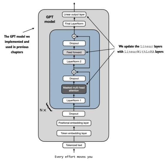
我們對使用 LoRALayer 取代原來的 Linear Layer: transformer 中的 Feed forward, attention block 的 K,Q,(and V?), 以及 output layer.

以下是需要修改的 code.

1 2 3 4 5 6 7 8 9 10 11 12 13 14 15 16 17 18 19 20 21 22 23

class LoRALayer(torch.nn.Module): def __init__(self, in_dim, out_dim, rank, alpha): super().__init__() std_dev = 1 / torch.sqrt(torch.tensor(rank).float()) self.A = torch.nn.Parameter(torch.randn(in_dim, rank) * std_dev) self.B = torch.nn.Parameter(torch.zeros(rank, out_dim)) self.alpha = alpha def forward(self, x): x = self.alpha * (x @ self.A @ self.B) return x class LinearWithLoRA(torch.nn.Module): def __init__(self, linear, rank, alpha): super().__init__() self.linear = linear self.lora = LoRALayer( linear.in_features, linear.out_features, rank, alpha ) def forward(self, x): return self.linear(x) + self.lora(x)

原始的 GPT2 model 是 124M.

1 2 3 4

total_params = sum(p.numel() for p in model.parameters() if p.requires_grad) print(f"Total trainable parameters before: {total_params:,}") Total trainable parameters before: 124,441,346

LoRA 的 trainable parameter: 1.3M. 比例只有 1%!.

1 2 3 4 5 6

replace_linear_with_lora(model, rank=8, alpha=8) total_params = sum(p.numel() for p in model.parameters() if p.requires_grad) print(f"Total trainable LoRA parameters: {total_params:,}") Total trainable LoRA parameters: 1,333,264

LoRA 的 accuracy ~ 98% 看起來還不錯！

1 2 3 4 5 6 7 8 9 10 11 12 13

from previous_chapters import calc_accuracy_loader train_accuracy = calc_accuracy_loader(train_loader, model, device) val_accuracy = calc_accuracy_loader(val_loader, model, device) test_accuracy = calc_accuracy_loader(test_loader, model, device) print(f"Training accuracy: {train_accuracy*100:.2f}%") print(f"Validation accuracy: {val_accuracy*100:.2f}%") print(f"Test accuracy: {test_accuracy*100:.2f}%") --------------- output ----------------- Training accuracy: 100.00% Validation accuracy: 96.64% Test accuracy: 98.00%

公佈答案

以下 7 个问题的答案：

1. 需要训练所有层吗？ NO, 可以用 PEFT.
2. 为什么微调最后一个 token，而不是第一个 token？
   1. BERT 是 bi-directional attention, 因此是用第一個 token
   2. GPT 是 causal attention, 需要用最後一個 token.
3. BERT 与 GPT 在性能上有何比较？差異不大
4. 应该禁用因果掩码 (causal mask) 吗？NO
5. 扩大模型规模会有什么影响？ Better
6. LoRA 可以带来什么改进？ 最好的 PEFT
7. Padding 还是不 Padding？NO

需要調整所有层吗？

出于效率原因，我们仅調整输出层和最后一个 transformer 块。如前所述，对于分类微调，无需更新 LLM 中的所有层。我们更新的权重越少，训练速度就越快，因为我们不需要在反向传播期间计算权重的梯度。

但是，你可能想知道如果不更新所有层，我们会留下多少预测性能。因此，在下表对所有层、仅最后一个 transformer 块（包括最后一层）、仅最后一层进行了微调。

結論：

1. 只調整最後一層的 output linear layer 雖然省計算，但精確度是遠遠不夠！
2. 加上最後一個 transformer block (1/12)，包含 attention layer and ff layer 則可以達到很好的效果。
3. 調整所有層效果最好，但只增加不到 2% 精確度，卻要多出 10 倍以上的計算量。

GPT-2 (124M)	All layers	Last block	Last layer
Training acc.	99.62%	96.63%	78.65%
Validation acc.	96.64%	99.33%	79.87%
Test acc.	96.67%	95.00%	72.00%

BERT

BERT（Devlin et al. 2018）等编码器式语言模型，你可能知道这些模型有一个指定的分类 token 作为其第一个 token，如下图所示：

![[Pasted image 20240929192333.png]]

BERT vs. GPT

BERT 和 GPT-2 124M 兩者差異不大。

SPAM Dataset	GPT-2 (124M)	BERT (340M)
Training acc.	99.62%	99.42%
Validation acc.	96.64%	99.33%
Test acc.	96.67%	97.67%

应该禁用因果掩码 (causal mask) 吗？

当我们在下一个词（next-word）预测任务上训练类 GPT 模型时，GPT 架构的核心特征是因果注意力掩码，这与 BERT 模型或原始 transformer 架构不同。

**但实际上，我们可以在分类微调阶段移除因果掩码， 从而允许我们微调第一个而不是最后一个 token。这是因为未来的 tokens 将不再被掩码，并且第一个 token 可以看到所有其他的 tokens.

不過不用 causal mask 沒有明顯的好處。不過可能會讓 program 比較簡單一點，因爲只要看第一個 token.

GPT-2 (124M)	Regular, Last block	W/o causal mask
Training acc.	96.63%	99.23%
Validation acc.	99.33%	98.66%
Test acc.	95.00%	95.33%

可以看到，在微调 (training) 阶段不用因果掩码 (causal mask) 可以带来略微的提升。但是在 validation 和 test 階段則是下降。基本是 overfit.

增加模型大小会带来哪些影响？

随着模型参数增加，预测准确率提升。不过 GPT-2 medium 是个例外，它在其他数据集上的性能同样很差。怀疑该模型可能没有经过很好的预训练。

![[Pasted image 20240929195627.png]]

Selective Fine-Tuning vs. LoRA 效果

我们需要训练所有层吗？结果发现，当仅仅微调最后一个 transformer 块而不是整个模型时， 我们可以（或几乎可以）匹配分配性能。所以仅仅微调最后一个块的优势在于训练速度更快，毕竟不是所有的权重参数都要更新。

LoRA 看起來效果不錯。可以看到，完整微调（所有层）和 LoRA 在数据集上获得了相似的测试集性能。

在小模型上，LoRA 会稍微慢一点，添加 LoRA 层带来的额外开销可能会超过获得的收益。但当训练更大的 15 亿参数模型时，LoRA 的训练速度会快 1.53 倍。

![[Pasted image 20240929213256.png]]

填充（Padding）还是不填充？

如果我們想要在訓練或推理階段用批次 (batch) 處理數據（包括一次處理多個輸入序列），則需要插入 padding token，以確保訓練樣本的長度相等。

![[Pasted image 20240929213815.png]]

图中描述了给定批次中的输入文本如何在 padding 过程中保持长度相等。

在常规文本生成任务中，由于 padding tokens 通常要添加到右侧，因而 padding 不影响模型的响应结果。并且由于前面讨论过的因果掩码，这些 padding tokens 也不影响其他 token。

但是，我们对最后一个 token 进行了微调。同时由于 padding tokens 在最后一个 token 的左侧，因此可能影响结果。

如果我们使用的批大小为 1，实际上不需要 pad 输入。当然，这样做从计算的角度来看很低效（一次只处理一个输入样本）。并且批大小为 1 可以用作一个变通方法，来测试使用 padding 是否影响结果。

可以看到，避免 padding tokens 的确可以为模型带来效果的显著提升。

![[Pasted image 20240929215405.png]]

但是在 mini-batch training 是需要加 padding, 因為每個句子的長短不同。而且根據 ChatGPT, padding and truncation 都是在左邊！原因如下！而且 padding 在左或右是 embedded in tokenizer (在 transformer 如此)。和 training or inferencing 無關。

Padding and truncation side decisions (left vs right) depend on the requirements of the model architecture and the specific use case. While right-padding and right-truncation are common defaults, there are valid reasons to use left-padding and left-truncation in specific scenarios.

Reasons for Left Padding and Truncation

1. Causal Language Models (e.g., GPT):

   • Models like GPT are causal language models that process input tokens in a left-to-right manner.
   • When padding or truncation occurs on the left, the most recent tokens remain at the end of the input sequence. This ensures that:
     • The model focuses on the most relevant context (e.g., for predictions in autoregressive generation).
     • The position embeddings align naturally with the most recent tokens.

2. Efficient Handling of Variable-Length Sequences:

   • In left-padding, the padding tokens (<pad>) occupy the beginning of the sequence. This reduces the computational burden during masked attention in autoregressive models because the padding tokens appear first and are easily ignored.
   • Truncating from the left ensures that the most recent or important context is preserved, which is critical in tasks where the end of the sequence carries the most significant information.

3. Token Position Alignment:

   • Models with absolute position embeddings (like GPT) rely on token positions being consistent. Padding on the left ensures the actual tokens align with their expected positions in the sequence.

4. Conversational Models:

   • In conversation-based tasks, truncating from the left keeps the most recent conversation turns, which are typically more relevant for generating responses.

5. Model-Specific Design:

   • Some models, particularly those trained with specific datasets or tasks, might expect input to be left-padded/truncated because that’s how they were trained.

---

Comparison of Left vs. Right Padding/Truncation

Aspect	Left Padding/Truncation	Right Padding/Truncation
Common Use Case	Autoregressive models (GPT)	Bidirectional models (BERT)
Focus on	Recent tokens	Earlier tokens
Attention Computation	Masked attention optimized for causal models	Generally applies to all tokens
Alignment with Outputs	Tokens align with expected positions	Positions shift due to padding/truncation

---

Key in the Code

The code snippet:

1 2 3 4 5 6

tokenizer = transformers.AutoTokenizer.from_pretrained( training_args.model_name, padding_side="left", truncation_side="left", ) tokenizer.pad_token = tokenizer.eos_token

indicates that the model is likely:

• An autoregressive model, where preserving recent context is more critical than earlier tokens.
• Handling conversational or sequential data, which benefits from left-side padding/truncation.

By setting padding_side="left" and truncation_side="left", the code ensures alignment with the model’s expected input format and optimizes attention computations.

Appendix A