Source

Medium by Oscar: LLM efficiency: https://axk51013.medium.com/llm-%E5%B0%88%E6%AC%84-%E8%A9%B3%E8%A7%A3-llm-inference-efficiency-32164c253627

LLM viewer!

【LLM 專欄】詳解 LLM inference efficiency

我們需要多少 GPU 來建立穩定的 LLM 服務？

倢愷 Oscar

Jul 27, 2025

這次來談一個筆者一年前就想寫也該寫的文章，但因為各種外務一直被延後 XD，也就是如何系統性分析 LLM inference efficiency。

到了 2025 年，企業內部部署 LLM 服務（如自建 ChatGPT 替代方案）已變得司空見慣。無論是銀行、醫療、電商，還是 SaaS 企業，許多組織都希望擁有一個私有的大語言模型（LLM），以便提供更可控、安全的 AI 服務。

這也帶來了一個關鍵問題：推理（Inference）成本正在成為 LLM 部署的主要瓶頸。相比 OpenAI 等雲端 API 提供商可以透過大規模 GPU 集群分攤成本，企業內部部署往往受限於固定算力，大多企業無法一次性購買大量 GPU，因此推理效率的優化變得至關重要。

更具挑戰的是，LLM 的應用場景正在從小規模的內部測試逐步擴展至大規模生產環境，從即時客服、內部知識檢索、程式碼輔助生成，到智慧分析與決策建議，每個場景對推理速度、吞吐量、延遲（Latency）和成本（Cost）都有不同的需求。如果推理效率不夠高，企業將無法在本地維持足夠的運算能力來支撐 AI 服務，甚至可能面臨算力成本失控的風險。因此，理解 LLM 推理過程，並探索如何優化其計算開銷，不僅關乎技術層面的實作，也將直接影響 AI 產品的可行性與競爭力。

⭐ 這些問題都是 LLM inference 的問題！一個好的 inference 架構，可以幫企業以更低的成本建立更好的服務⭐

這篇文章打算依序回答幾個問題：

LLM inference 到底發生了甚麼事情？
當我們部屬一個 LLM 服務時，我們如何 ”正確” 預估我們所需要的 GPU 量。
如何判斷我們現在的 latency bottleneck 是什麼？

幫助大家更好的建立企業內的 inference 架構，提升企業內的服務穩定性、GPU 利用率。

0. Preliminary: LLM inference 的時候到底發生了甚麼事情

⭐ Part1: Decoder only Transformer 的正向傳導（forward pass）

要討論 inference 的效率之前，最最最基本的就是要先了解 Decoder only 的 Transformer 一次正向傳導（forward pass）具體計算了甚麼。

也就是理解以下這張圖每一個 components 的運作方式。

Press enter or click to view image in full size

image from [1], 說明 GPT 跟 LLaMA 的架構差異，以及具體的運算

實際上相關的知識已經有非常多很好的教學、文章可以參考，筆者也沒有自信可以找到一個新的角度或是寫得更清晰，所以推薦大家可以去閱讀以下這些經典教學文章：

Harvard The Annotated Transformer
Andrej Karpathy Let’s build GPT: from scratch, in code, spelled out.
Stanford CS336: Language Modeling from Scratch [課程網站][簡報][課程影片]

為了方便後續理解，筆者還是把我認為重要的幾個觀念以筆者的思路記錄下來，只要看得懂以下的段落應該就可以順暢理解本文的重點。

1️⃣ LLM 一次正向傳導（forward pass）主要的參數與運算成本（FLOPs）聚集在 attention 跟 FFN 層。

如果我們以 GPT2 當作範例，從 input 到 output 依序會經過許多操作（如下圖）

Press enter or click to view image in full size

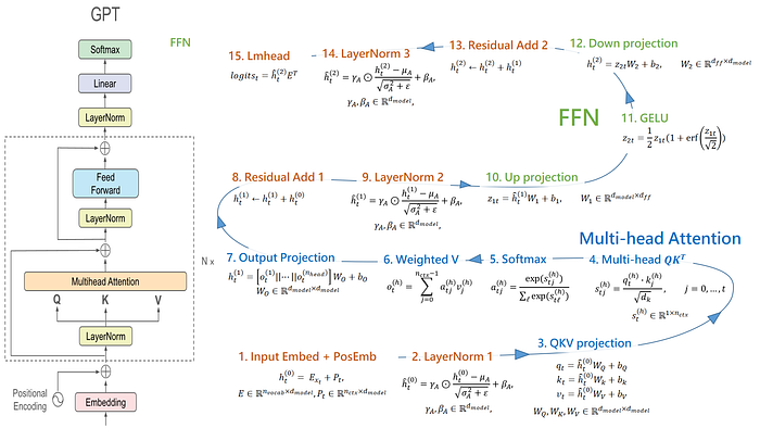
figure: GPT-2 架構具體的運算過程，這邊為了方便討論我們假設 N = 1，也就是單層的 GPT-2 架構。

如果我們把這裡每一個運算具體的參數量以及每 forward 一個 tokens 的運算量（FLOPs）依序精準算出，會如下表。

Press enter or click to view image in full size

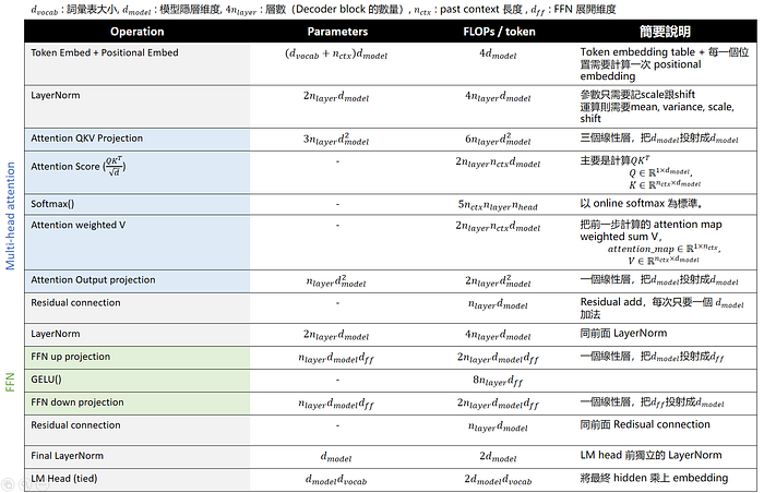
Table: GPT-2 架構下每一層的參數量（Parameters）跟運算量（FLOPs/token）

如果打算深入 LLM 的 High Performance Computing，請務必保證自己對上表的每一個公式了然於心，因為上表會是我們後續分析的基石。

接著我們可以帶入數字來討論，以 GPT-2 small 為例。

gpt2_small_cfg = dict(
d_model = 768,
n_layer = 12,
d_ff = 3072,
n_ctx = 1024,
d_vocab = 50257
)

計算出來結果會如下表。注意我們這邊在計算 FLOPs 的時候統一把 matrix multiplication 中每一個 element 的乘法當作 2 個運算（Multiply 跟 Accumulation），這種算法是參考 OpenAI 的計算方法 [2]，筆者認為也是當下 LLM community 的共識算法。

Press enter or click to view image in full size

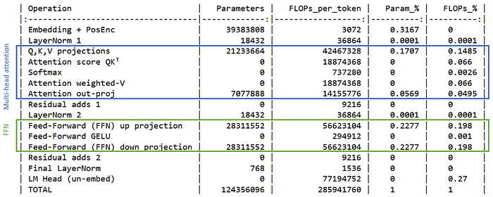
figure: gpt-2 small 統計參數量、Flops per tokens

可以看到，不論是從參數量（Paramters）還是運算量（FLOPs）的角度，attention 以及 FFN 都佔據主軸，而 LayerNorm, Residual Connection 則完全不重要（甚至在四位小數的精度下被捨去）。

唯一不是 attention 跟 FFN 但參數量一樣重要的是 input embedding + PosEnc 層，而唯一不是 attention 跟 FFM 但運算量一樣重要的是 LM head。

❗需要特別注意，因為 GPT-2 的 LM head 跟 input embedding 是 tie embedding，所以我把 LM head 的參數量記為 0，因為這組參數在 input embed 層已經記過。但實際上只是帳記在哪的問題，而在進行運算的時候我們還是都要送到 GPU SMs。

雖然在 GPT-2 small 看起來 input embedding 跟 LMhead 也很重要，但實際上因為 input embedding 跟 LMhead 都是一次性的操作（跟模型層數無關），所以隨著模型變大變深，這兩個影響會越來越小。下圖我把 gpt-2 的 4 種大小（small, medium, large, XL）都計算出來，可以看到到 GPT-2 large 以後，input embed 跟 LM head 的影響都不到 10% 了，GPT-2 XL 則只有 4~5%。

Press enter or click to view image in full size

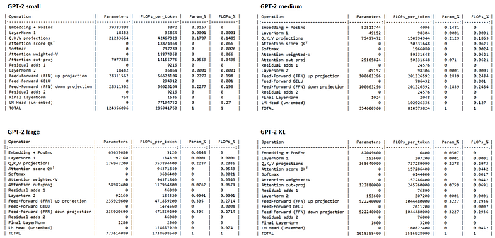
figure: 不同大小的 gpt-2 的參數量以及 FLOPs per token

如果我們討論到 7B 甚至更大的模型，LM head 跟 input embed 則大多時候完全可以不用討論。

🔥 這裡我們得到第一條結論：LLM 一次正向傳導（forward pass）主要的參數與運算成本（FLOPs）聚集在 attention 跟 FFN 層。🔥

因此我們後續為了討論的簡潔性，大部分時候我們會只討論 Attention 跟 FFN 帶來的影響，而忽略其他層的參數、運算量。

2️⃣ Attention 的運算量（FLOPs）隨著序列長度二次（Quadratic）成長並且迅速 Dominate 整體運算量。

接下來我們來更仔細來看 attention 跟 FFN 的運算量（FLOPs），來看看到底哪一個運算才是主要帶來延遲（Latency）的元兇。

有學過 Transformer 的人可能都有聽過一句話：Transformer 是 Quadratic complexity。尤其在 2023 Mamba [3] 特別紅的那段時間，大家都會比較 SSMs, Linear transformer, RNN 跟標準的 Transformer，大多都會提到 Transformer 最大的壞處就是 Quadratic complexity。

但是這個 Quadratic complexity 到底是在說甚麼？

回頭來看我們一開始的 Table，會發現其中 Attention 有 3 個項目的運算量（FLOPs）會依賴 n_ctx 這個參數。

Press enter or click to view image in full size

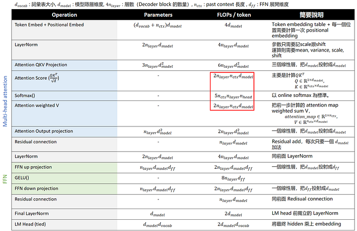
image: 在 Multi-head Attention 的計算中，Attention score (QK), softmax跟 Attention weighted V 會依賴於歷史資訊，因此運算量會跟 n_ctx 正比

也就是說每次 forward 一個 token（生成一個 token）的運算量會跟這個 token 之前的 context 長度有關，是 O(n_ctx) 的操作。

❗ 後續為了簡化討論，忽略不占運算量、參數量的運算，包含 Attention 中的 softmax 跟 FFN 中的 GELU

Press enter or click to view image in full size

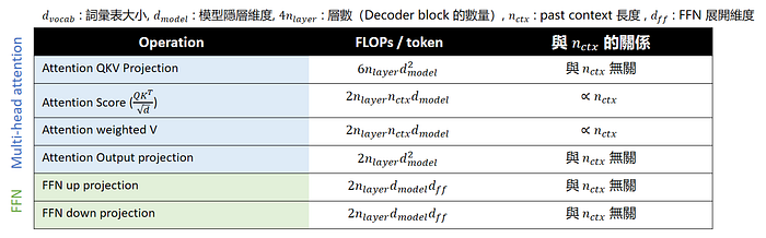
單獨把 attention 跟 FFN 層拉出來討論，觀察與 n_ctx 的關係

因為每生成一個 token 就會是一次 O(n_ctx) 的操作，把「對每個 token 進行一次」的動作加總到整段序列（總共最終生成出 n_ctx 個 token），就會形成熟悉的 O(n_ctx²)，這就是大家口中的 Quadratic complexity。

但我們在做 DL 的時候，complexity 只是一個參考，我們通常更注重實務上具體的情況，因此其實我們更在意的是「何時 Attention 的運算量會超越 FFN」以及「什麼時候 Transformer 會呈現二次性」

第一、何時 Attention 反超 FFN？

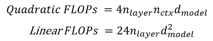
為了量化「哪一個運算主宰延遲」，可以把兩者的 FLOPs 拿來做不等式比較。以 GPT‑2 small 為例（d_model = 768，d_ff = 3072，n_layer = 12）：

Press enter or click to view image in full size

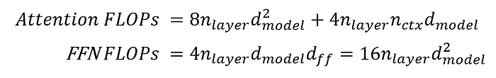
其中因為 GPT-2 的 d_ff 統一都設定成 4 * d_model，所以 FFN FLOPs 我們可以把 d_ff 全部換成 4 * d_model 來表示。

令兩者相等即可得到臨界點 n*:

Press enter or click to view image in full size

n_ctx < 1536 時：FFN 仍是主要的計算瓶頸。
n_ctx > 1536 時：Attention 的計算量就會超過 FFN。

若代入 GPT‑2 medium 的參數（d_model = 1024，d_ff = 4096，n_layer = 24），臨界點變為 2048。

而現在的大模型動輒就宣稱 128k context 甚至是 1M context，因此在長文本情景下確實更容易變成 Attention 為主要運算量。

第二、什麼時候 Transformer 會呈現二次性

前面只是說明 Attention 在 n_ctx 超過 2 * d_model 才會開始主導整個運算量，但我們更在意的可能是什麼時候開始出現二次性（Quadratic Complexity）。

二次性主要的來源就是跟 n_ctx 相關的操作，如果有一個操作每次處理一個 token 的運算量都跟 past context length 線性，總共會生成 N 個 token（input prompt + output），每一個 token 都需要 n_ctx 個運算，整體運算量則會呈現 n_ctx * n_ctx 複雜度，因此會跟 context length 成二次關係。

因此我們把 Attention 跟 FFN 中跟 n_ctx 相關的運算量定義為 Quadratic computation，並比較 Quadratic computation 跟 Linear computation 的運算量。

Press enter or click to view image in full size

一樣令兩者相等即可得到臨界點 n*:

Press enter or click to view image in full size

在 GPT-2 small 的架構下（d_model = 768，d_ff = 3072，n_layer = 12）：

n_ctx < 4608 時：Transformer 主要呈現跟 n_ctx 線性的運算量。
n_ctx > 4608 時：Transformer 主要呈現跟 n_ctx 二次性的運算量。

🔥 因此不論是哪一個運算，都告訴我們隨著 n_ctx 變長（也就是 input token + 過去的 decode token 越多），Attention 會快速 dominate 整體運算量，並讓 LLM 呈現出二次性。

Press enter or click to view image in full size

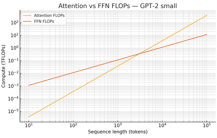
隨著長度變長，Attention 占的運算量會快速 dominate 整體運算。

我們也可以跟總體運算量相比，可以看得更清楚到一定長度後運算量（FLOPs）幾乎就是以 Attention 為主。

Press enter or click to view image in full size

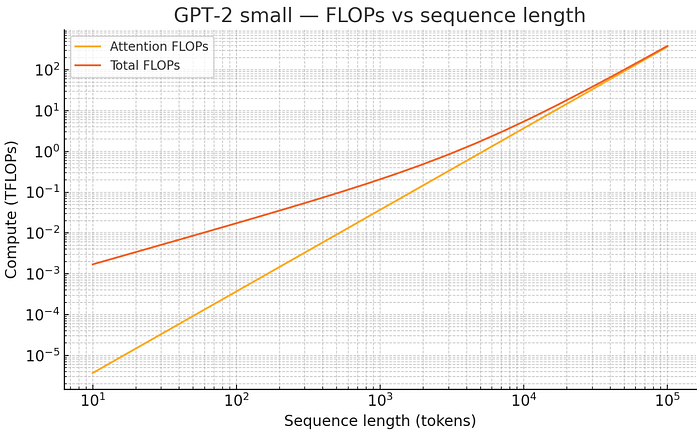
image: 比較總體運算量（Total FLOPs）跟 Attention 的運算量（Attention FLOPS），可以看到隨著長度變長，Attention 佔比急劇上升。

所以這裡是我們第二個重要結論：隨著 n_ctx 變長（也就是 input token + 過去的 decode token 越多），Attention 會快速 dominate 整體運算量，並讓 LLM 呈現出二次性。

3️⃣ LLM 一次正向傳導（forward pass）所需要的運算量，近似於兩倍參數量（2N）。

接著我們想要一個公式估算我們每一次的正向傳導（forward pass）精準所需的運算量（FLOPs），我們一樣把前面表格攤開，並且只關注 Multi-head Attention 跟 FFN 的部分，如下表。

Press enter or click to view image in full size

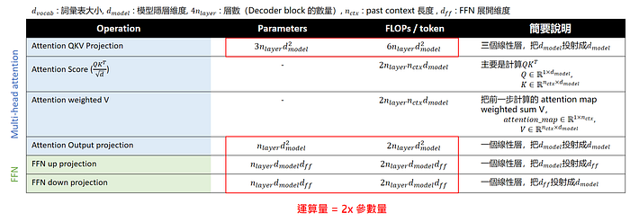
可以馬上發現除了計算 Attention Score 跟 Attention weighted V 這兩步以外，其他部分的運算量都剛好是 2x 參數量。（其實也不是剛好，大家可以想想為甚麼會有這種結果）

因此過去很多人會直接用 2N（N = 模型參數量）來近似一次正向傳導（forward pass）所需的運算量。

不過我們這邊力求精準，我們把那兩項也帶上，每一次正向傳導（forward pass）變成 2N + 4 * n_layer * n_ctx * d_model。

但實際上到這邊還是沒有結束，如果我們整個 context 最後長度是 K，實際上並不是每一個 token 都會 attend 到所有的 K 個 tokens，因為現在的 LLM 主要都是 Causal LLM。

意思是每一個 token 只會看到前面的 tokens，而不會看到後面（未來）的 tokens，實作上我們是套用一個 causal mask，來遮蓋住未來的資訊，如同下圖

Press enter or click to view image in full size

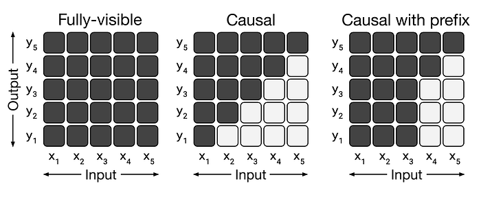
參考中間 Causal 的圖示，y5 生成時能參考 x1~x5，而y4 只能參考 x1~x4，y3 參考 x1~x3 以此類推，每一個 query 只參考過去的 key ，而不關注未來。

因此加入 causal 的考量，假設我們 input + output token = n_ctx，我們實際每一個 token 平均只需要 2N + 2 * n_layer * n_ctx * d_model 個運算量即可，因為平均每個 token 只會參考一半的過去 tokens（0.5 * n_ctx）。

🔥 平均每一個 token 的運算量 = 2N + 2 * n_layer * n_ctx * d_model

❗實際上這個算法我認為是大有爭議，畢竟我們實際操作上並不會真的減少運算量，而是透過 mask 的方式操作，但因最早 OpenAI 是這樣算，所以大家也習慣變成這樣算。當然現在也有真正 triangular GEMM 的 kernel，這個我們之後有機會再談。

好！到這裡我們藉由 GPT-2 的案例清晰說明了 decoder only 的 transformer 一次正向傳導（forward pass）具體發生甚麼事，並且藉由對每一個運算的清晰了解，我們得出了 3 個重要觀念。

LLM 一次正向傳導（forward pass）主要的參數與運算成本（FLOPs）聚集在 Attention 跟 FFN 層。
Attention 的運算量（FLOPs）隨著序列長度二次（Quadratic）成長並且迅速 Dominate 整體運算量。
平均每一個 token 的運算量 = 2N + 2 * n_layer * n_ctx * d_model

實際上同樣的分析也可以套用在任何你知道的 LLM 架構中，也確實有人這樣做了，Yuan, Zhihang, et al [4] 基於一樣的分析方式，發表了 LLM Viewer [4]，提供了多種主流模型的具體分析程式（llama2, opt, chatglm, gpt-j）。

同時他還有參考一些主流的運算方式，像是 attention 主流會採取 flash attention v2 的運算方式，進而做更精確的估算。

我自己工作中因為需要清晰分析每一個模型的運算量，我也基於 LLM Viewer 這個專案去改出了可以兼容更多模型（llama3, qwen2.5, qwen3, deepseek v3, …）的程式，不過核心觀念其實就是我前文列出的 table，如果你針對每一個模型都能精準寫出對應的參數量（parameters）跟運算量（FLOPs），那具體寫成程式甚至可以交給 ChatGPT 來負責即可。

⭐ Part2: LLM completion 過程：Prefilling vs Decoding

了解一次正向傳導（forward pass）具體的細節後，那我們就要把視角拉高一點，來討論一次 LLM completion 具體發生什麼事。

LLM completion 其實就是丟入一組 prompt，然後讓 LLM 做接龍（next word prediction）直到 LLM 輸出結束符號（eos token）。

而 chatcompletion 其實只是在接龍的模板上加入某些對話的標記（apply chat template），並且讓在 instruction finetuning 的時候特別訓練 LLM 去基於 input prompt 回答問題或是執行指令。

Press enter or click to view image in full size

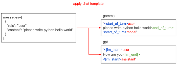
所以不論是 completion 還是 chatcompletion 其實都包含兩個過程：

Prefilling：LLM 閱讀理解 input prompt。
(Auto-regressive) Decoding：LLM 做 next word prediction 直到結束（輸出 eos token）。

不過這個說法其實還是比較「直覺想問題」，讀過筆者較多文章的朋友應該都知道筆者最排斥的就是用直覺想問題，很多事情我們把公式攤開才可以更清晰討論。

🔥 我們先來討論一個簡單的問題：LLM 到底什麼時候會用到「歷史資訊」？又是怎麼用的？

人類在閱讀時，眼睛滑過每一行文字，都會把新線索連同舊線索一起丟進腦海更新「情節模型」 — — 這讓我們隨時知道角色是誰、事件怎麼發展。如果我們希望 LLM 具備類似人類的閱讀理解能力，那 LLM 必定也要以某種方式「使用歷史資訊」。

我們知道 LLM 在輸出每一個 token 的時候，需要先後經過大量的 Attention 跟 FFN，那我們就來重點關注 Attention 跟 FFN 的哪些操作牽扯到了歷史資訊。

下表我們依照前文的表格，把 Attention 跟 FFN 具體的運算過程列出，如下表。

Press enter or click to view image in full size

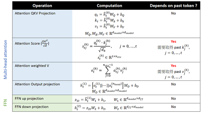
可以清晰看到，在整個 Attention 跟 FFN 中，只有 Attention 的兩步跟歷史資訊有關，第一步是計算 Attention score，計算當下 query 跟每一個歷史的 key 的相關性，第二是拿 softmax 後的 attention score 去跟每一個歷史的 Value vector 做加權。

因此可以清晰看見 Transformer 在閱讀的時候，主要就是把資訊保存在 key/value vector 中，提供後續的 query 使用，而這也就是俗稱的 KV cache。

🔥 KV cache：歷史的 Key/Value Vector，用來保存歷史資訊，提供後續 token 計算 Attention 時使用。

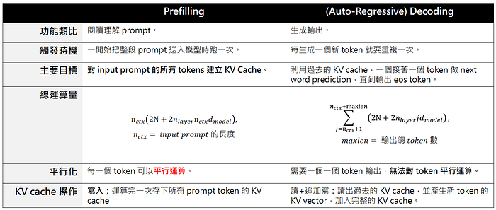
理解了 KV cache，我們就能更清晰整個 LLM 的 completion 過程，其中 Prefilling 跟 Decoding 的差異：

Prefilling：LLM 閱讀理解 input prompt，產生 KV cache 提供給後續 Decoding 使用。
(Auto-regressive) Decoding：基於過去 KV cache ，LLM 一個一個 token 接續做 next word prediction ，每一個輸出 token 當作下一個 input token，直到結束（輸出 eos token）。

Press enter or click to view image in full size

image from [5]，講解 prefilling 跟 decoding 的概念，可以看到 Prefilling 計算出來的 KV cache 會持續給每一步的 decoding 使用。

而因為 Prefilling 的主要目的就是產生所有 input prompt 的 KV cache，因此在 Prefilling 的過程中我們可以平行處理所有的 input prompt tokens。

綜上所述，我們可以把 LLM completion 的過程分成 Prefilling 跟 Decoding 兩個階段，Prefilling 藉由大規模平行，來高效閱讀/理解 input prompt 並產出 KV cache，再交由 Decoding 來生成輸出，而 Decoding 會一個接著一個 token 生成。細節如下表

Press enter or click to view image in full size

好目前我們對 LLM 一次正向傳導（forward pass）已經了解，也理解了一次 completion 的 prefilling 跟 decoding，接下來就是我們的正餐，來分析 LLM 運算效率，藉此來確定我們該使用的硬體設置。

1. 評斷 LLM 的運算效率 Roofline Model and Arithmetic Intensity

前文帶大家比較細緻的理解基礎 LLM completion 的過程，接下來要來討論我們的分析框架，怎麼樣分析每一個操作在 GPU 上面的效率。

1️⃣ Arithmetic Intensity

Arithmetic Intensity (AI) = 浮點運算次數 (FLOPs) / 記憶體存取量 (Bytes)

Arithmetic Intensity 描述的是在執行一段程式碼時，每存取 1 Byte 資料所能完成的運算量。對 GPU 而言，Arithmetic Intensity 是判斷運算核（kernel）是受到運算吞吐量（GPU Computation）或記憶體頻寬（GPU Memory Bandwidth） 限制的關鍵指標。

🔥 那 Arithmetic Intensity 對我們有什麼用處？

🔥 答：Arithmetic Intensity 可以用來判斷「特定運算」在「特定 GPU」底下是 Computation Bound 還是 Memory Bandwidth Bound。🔥

舉例而言我們來看 H100 的 datasheet。

Press enter or click to view image in full size

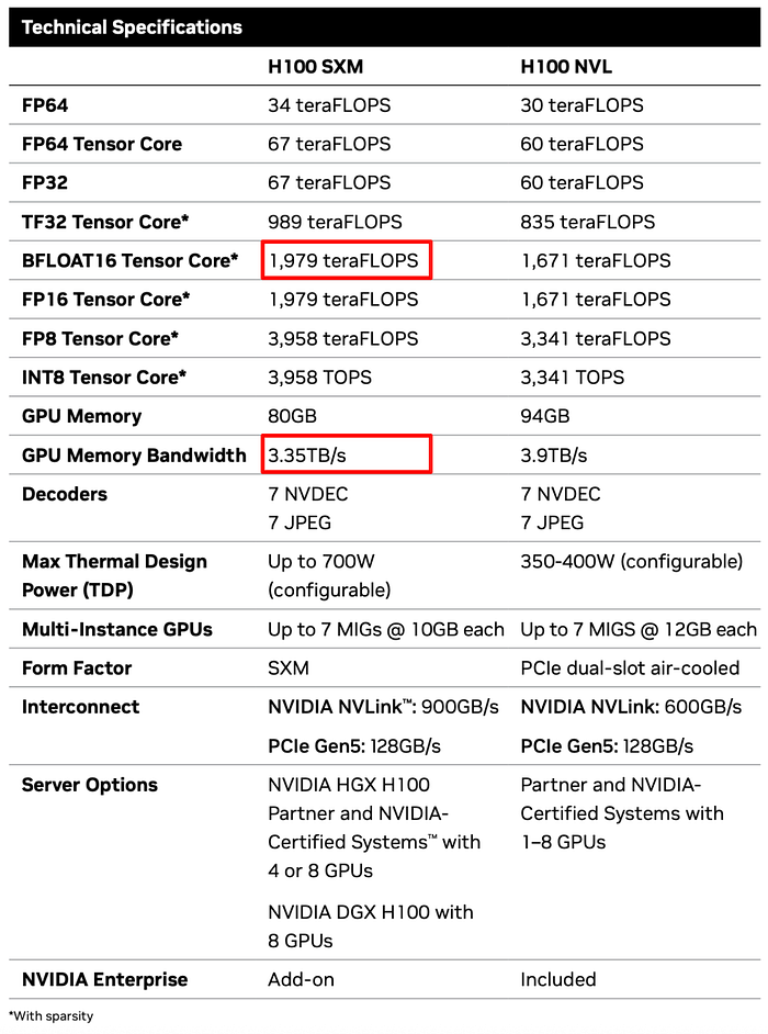
image: H100 datasheet https://www.nvidia.com/en-us/data-center/h100/

用紅框框出來的兩個數字就是我們用來算 H100 Critical Arithmetic Intensity 的數值，也就是 H100 到底每一個 Bytes 要做多少 BF16 的運算（FLOPs），才能用滿 H100 computation。

為什麼是看 BF16 Tensor Core？因為目前 LLM 主流都使用 BF16 精度。

同時需要特別注意，從 A100 以後 Nvidia 的 datasheet 預設都標 2:4 sparsity 的運算量（意思是每 4 個 bits 有最少 2 個 0，因而可以加速），但我們在 inference 或 train LLM 的時候極少會開啟 2:4 sparsity，所以我們實際可用數值還要除 2，也就是 1979 TFLOPs/2 = 989 TFLOPs。

所以 H100 SXM 的 Critical Arithmetic Intensity = 989 TFLOPs / 3.35 TB/s = 295。

也就是說，如果特定運算的 Arithmetic Intensity = C，

若 C ≪ 295，效能被 H100 記憶體頻寬（Memory Bandwidth）限制；無法用滿 H100 的運算能力，也就是 Memory Bandwidth Bound。
若 C ≫ 295，Kernel 已受計算峰值限制；用滿 H100 的運算能力，也就是 Computation Bound。

接著我們來看幾個運算：

➕ 矩陣加法：假設兩個 N * M的矩陣（elementwise）相加在一起，得出一個 N * M 的輸出矩陣。

Press enter or click to view image in full size

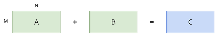
我們來分析矩陣加法的 Arithmetic Intensity：

運算量（FLOPs）：總共需要 N * M 個加法，每 1 個加法需要 1 個 FLOP，總共是 N * M FLOPs。
Memory IO（Bytes）：分別需要把 A 跟 B 兩個矩陣寫入，並把 C 寫出，所以需要 3 * N * M * 2 Bytes（BF16 底下每一個 parameter 占 2 Bytes），總共是 6 * N * M Bytes。

🔥 Arithmetic Intensity = FLOPS / IO = (N * M) / (6 * N * M) = 1/6

接著我們帶入幾種組合，可以得到下表。

Press enter or click to view image in full size

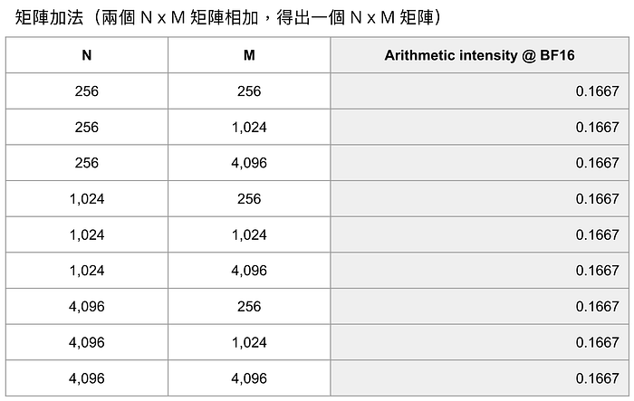
也就是說矩陣加法，不論矩陣的維度，永遠 Arithmetic Intensity = 1/6。

因為 1/6 ≪ 295，所以矩陣加法是絕對的 Memory Bandwidth Bound，無法利用好 H100 的運算資源，主要都在等資料搬運。

✖️ 矩陣乘法：假設一個 N * K 的矩陣乘上一個 K * M 的矩陣，得出一個 N * M 的輸出矩陣。

Press enter or click to view image in full size

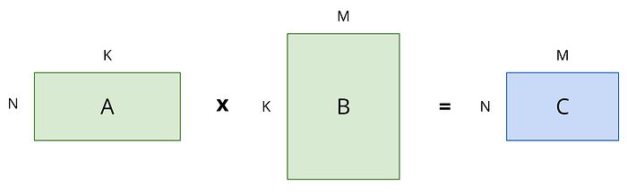
我們來分析矩陣乘法的 Arithmetic Intensity：

運算量（FLOPs）：總共需要 N * K * M 個矩陣 element 相乘，每 1 個 element 相乘需要 2 個 FLOPs（Multiply + Accumulation），總共是 2 * N * K * M FLOPs。
Memory IO（Bytes）：分別需要把 A 跟 B 兩個矩陣寫入，並把 C 寫出，所以需要 (N * K + K * M + M * N) * 2 Bytes（BF16 底下每一個 parameter 占 2 Bytes）。

🔥 Arithmetic Intensity = FLOPS / IO = (N * K * M) / (N * K + K * M + M * N)

接著我們帶入幾種組合，得到下表。

Press enter or click to view image in full size

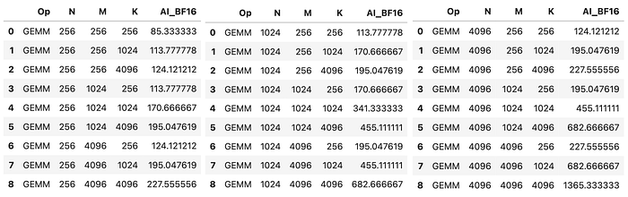
可以看到矩陣乘法的 Arithmetic Intensity 顯著較高，並且隨著維度越大整體還會越大，顯示出矩陣乘法比矩陣加法更能良好運用 GPU 的運算資源。

如果 N, M, K 都是 4096 更可以達到 1365 這種數字，超過 H100 的 Arithmetic Intensity 295 一大截，可以完美使用 H100 的運算資源。

從矩陣乘法跟矩陣加法我們可以很清晰看出，不同運算對於 GPU computation 的利用率是可以天差地別的，如果我們希望我們最有效使用 GPU，則應該讓我們的運算的 Arithmetic Intensity 盡量超越我們所使用 GPU 的 Critical Arithmetic Intensity，才可以用滿 GPU 的大規模平行運算能力。

2️⃣ Roofline Model

而基於 Arithmetic Intensity，大家又更開發出一個視覺化的分析模型：Roofline model（屋簷模型），幫助簡化理解。

Press enter or click to view image in full size

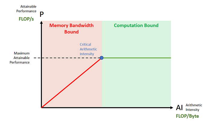
image: roofline model 紅色的區域因為還沒有達到 critical arithmetic intensity，因此還是 memory bandwidth bound，無法用滿 computation，而綠色的地方則因為已經超過 critical arithmetic intensity，而是 computation bound，在該 GPU 上已經用滿所有運算能量。

Roofline model 用清晰的圖像來把剛剛複雜的邏輯表示清楚，如果運算的 Arithmetic Intensity 比 Critical Arithmetic Intensity 小，我們都處於 Memory Bandwidth Bound，GPU 都在等待資料搬運，而無法用滿 GPU 的運算資源。而如果運算 Arithmetic Intensity 比 Critical Arithmetic Intensity 大，我們則處於 Computation Bound，GPU 都在等運算。

Get 倢愷 Oscar’s stories in your inbox

Join Medium for free to get updates from this writer.

來看一下我們熟悉的不同 GPU 的 roofline models，包含 H100, A100, A6000, 5090, 4090，取 Nvidia 官網公告的數字計算後，以 BF16 tensor core dense computation 為標準，分別的 roofline model 如下圖。

Press enter or click to view image in full size

可以看到這些 GPU 的 Critical Arithmetic Intensity 大約都在 100~300 上下，以 H100 的 295 最高，意思是如果我們可以保證我們大部分運算的 Arithmetic Intensity > 300，那在主流 GPU 上我們都可以用好用滿運算資源。

可以注意 H100 不論是 Critical Arithmetic Intensity 或是 Maximum Attainable Performance 都顯著優於其他選擇，Hopper 架構相較於 Ampere 還是有滿多提升（這個之後再提）。

再來看同樣都是 H100，不同精度的 Roofline model 又會有什麼差別，如下圖。

Press enter or click to view image in full size

可以看到精度越低，因為 GPU 運算能力越強，所以得到的 Critical Arithmetic Intensity 也越高，越能做 Computation intensive 的任務，像是高維度的矩陣乘法。這也是為什麼每一代 Nvidia 都要強調新的低精度運算（Hopper 強調 FP8、Blackwell 強調 FP4）。不過實際上因為精度變低，IO 也會相對應的變低（要運的資料變輕了），所以在大部分未經過優化的運算上其實影響不大，更大的優勢是來自於本身低精度的運算效率提升。

好！現在我想大家都能比較直觀理解 Arithmetic Intensity 跟 Roofline Model 了，那我們就來利用這些觀念，來預估 LLM inference 的 Latency。

2. LLM inference Latency 估計

前文中我們已知 LLM completion 具體會分成 Prefilling 跟 Decoding 兩個步驟。

接下來我們要先來分析 Prefilling 跟 Decoding 分別是 Memory Bandwidth Bound 還是 Computation Bound。

我們一樣以 H100 的 Critical Arithmetic Intensity = 295 來討論，已知 Prefilling 可以把所有 token 平行運算，

運算量（FLOPs）：總共 n_ctx 個 token 需要平行處理，每一個 token 平均需要 2N + 2 * n_layer * n_ctx * d_model。
Memory IO：總共要送入一份 Model Weight，送入所有 token 的 input id 以及存出 Output KV cache。

因此 Prefilling 的 Arithmetic Intensity 會如下圖

Press enter or click to view image in full size

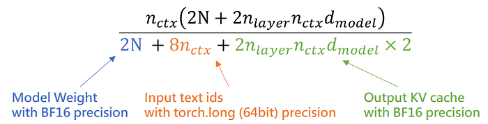
Prefilling Arithmetic Intensity，其中特別注意 KV cache 最後還有一項 *2，是因為同時要存 Key 跟 Vector 兩組。

其中 input prompt id 的佔比幾乎可以忽略，所以我們化簡後就可以得到 Prefilling 的 Arithmetic Intensity ~= n_ctx。

input prompt 長度 ≫ 295 時，就可以用滿 H100 的 computation resource，變成 computation bound。
input prompt 長度 ≪ 295 才會是 Memory bandwidth bound。

❗注意：我們這裡用整理運算量跟整體 Memory IO 來估計一定是不準確的，更精準需要逐層分析，但整體分析可以快速帶給我們直觀理解。

🔥🔥 而我們現在大部分的應用 prompt 長度 ≫ 295 都是常態，所以我們幾乎可以說 prefilling 正常情況下都是 computation bound。

接著來看 Decoding，已知 Decoding 要一個接著一個 token 來（Auto-regressive），因此我們不能對 tokens 平行處理，只能討論單一 token 的情況

運算量（FLOPs）：每一個 token 平均需要 2N + 2 * n_layer * n_ctx * d_model。
Memory IO：總共要送入一份 Model Weight，送入過去所有 token 的 KV cache，存出 Output KV vector，以及存出 output token id。

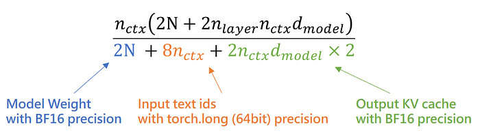
因此平均一個 token 的 Arithmetic Intensity 則如下，這裡的 n_ctx 指的是 input + output 長度，

Press enter or click to view image in full size

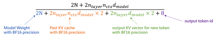
Image: Decoding Arithmetic Intensity

可以看到，Decoding 的 Arithmetic Intensity，不論模型大小、context 長度，都會是一個接近 1 的數字。

也就是說除非我們把 concurrent batch 開很大（同時送入很多 decoding requests），不然 Decoding 永遠都是 Memory Bandwidth Bound。

⭐Prefilling 大多時候是嚴格的 computation Bound，Decoding 大多時候是嚴格的 Memory Bandwidth Bound。

接下來我們要延續這個結論，進一步分析 Prefilling 跟 Decoding 的 Latency。

1️⃣ Prefilling Latency 分析

因為 Prefilling 是 Computation Bound，所以我們可以把 Prefilling 的 Latency 寫成以下這個公式：

Press enter or click to view image in full size

理論的 Prefilling latency，分子是 prefill 完整 prompt 所需運算量（FLOPs），分母就是你所使用的 GPU 的 computation 能量（FLOP/s）

假設我們把這個公式代入 H100 的數字，以及 LLaMA-3.1 的模型架構，我們先討論 prompt 長度 < 4k 的範圍內，我們可以看到 theoretical prefilling latency 如下圖。

Press enter or click to view image in full size

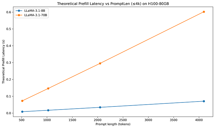
在 computation bound 的情況下，prefilling 需要的 computation 會跟 prompt length 成正比，因此 prompt length 越長，Theoretical latency 就會線性上升。

可以看到因為 prompt 長度 ≫ 295，所以已經到 computation bound，更多的 prompt tokens 進來只能等 GPU 資源釋出，因此 prompt 長度跟 theoretical prefill latency 成線性關係。

如果今天把 prompt 長度 > 4k 的範圍也拉進來，則會畫出下圖。

Press enter or click to view image in full size

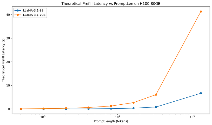
當 prompt length 較長的時候，因爲二次項變得主導，因此會開始出現二次性。

可以看到到 32k, 64k, 128k 的時候， theoretical prefill latency 就開始出現二次性，如同前文所說，當 context 較長時，Transformer 才會出現二次性。

因此其實如果我們動輒就撰寫 64k 甚至更長的 prompt，其實會大幅度影響到我們的 prefilling latency。

而如果我們比較不同 GPU，也可以很清晰看到因為 H100 的 maximum attainable performance 比 A100 高許多，所以 H100 的 Latency 會顯著低於 A100，如下圖。

Press enter or click to view image in full size

H100 因為 computation performance 顯著高於 A100，所以對應的 Theoretical prefilling latency 也都顯著低於 A100。

2️⃣ Decoding Latency 分析

因為 Decoding 是 Memory Bandwidth Bound，所以我們可以把 Decoding 的 Latency 寫成以下這個公式：

Press enter or click to view image in full size

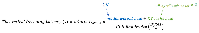
理論的 Decoding latency，分子是 decoding 一個 token 所需搬運的主要資料大小，分母就是你所使用的 GPU 的 Memory Bandwidth（Bytes/s）

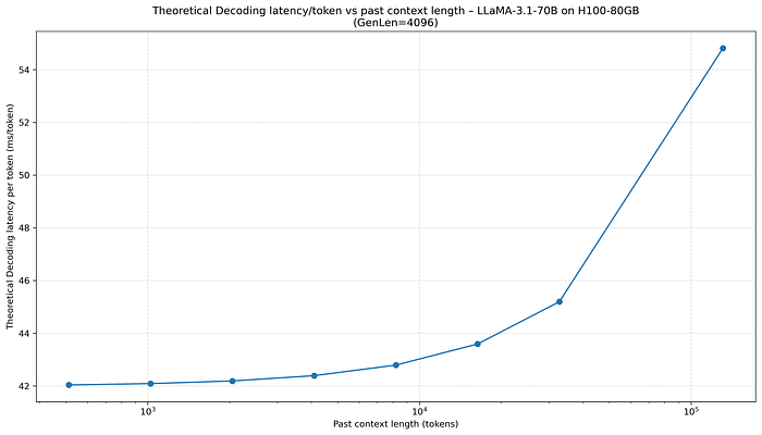
假設我們把這個公式代入 H100 的數字，以及 LLaMA-3.1 的模型架構，我們先討論 past context長度 < 4k 的範圍內，我們可以看到 theoretical decoding latency 如下圖。

Press enter or click to view image in full size

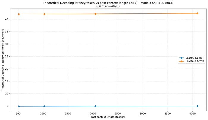
在 past context length 較短（<4k）的前提下，decoding latency 會很接近恆定，因為我們主要的 IO bottleneck 是運送 model weight 而不是運送 KV cache，所以整體 IO 接近常數。

在 4k 的範圍內，不論 past context 長度怎麼更改，都幾乎不影響 latency，因為在 past context長度較短的時候，主要要搬運的就是 Model weight，因此各個 past context長度跑出來的數據差不多。

如果我們把 past context長度開放到 128k，則會開始有差，因為這時 KV cache 的大小開始佔比越來越大。

Press enter or click to view image in full size

當 past context length 開始上升，甚至到 128k，因為 KV cache 變大許多，所以整體 IO 也會跟著提升，進而增加 Decoding Latency。

對於 LLaMA-3.1–8B，當歷史 context 長度變長，KV cache 造成的影響會更顯著（如下圖，重點關注縱軸的差異，可以看到 Theoretical Decoding Latency 到 128k 長度時接近翻倍）。

Press enter or click to view image in full size

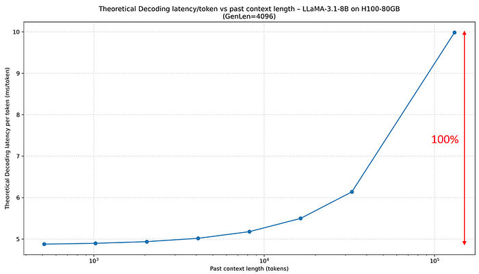
LLaMA3.1–8b 因為 KV cache 佔比較大，所以 past context length 拉長後對 latency 的影響更大。

主要的變因是 LLaMA 8b 模型的 GQA Group 比例比 70b 模型更低，但這個較複雜我們之後會談。

如果我們把尺度再放更大，討論到 past context length 有可能到一百萬長度，KV cache 佔整體 IO 的比例就會顯著上升。

Press enter or click to view image in full size

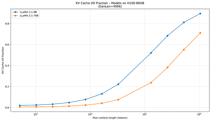
當我們考慮到 1M context length 時，KV cache 就幾乎主導 IO

3️⃣ Maximum Concurrent Requests

目前的分析框架除了能提供我們 Prefilling 跟 Decoding 的 Theoretical Latency 以外，其實還能幫助我們了解硬體限制上的最大 concurrent requests。

在大部分的 Deep Learning 運算中，嚴格限制了 max concurrent requests 的因素通常都是 GPU Memory，只要你所需要運算的 data 放的進 GPU Memory 裡面，不論是 GPU computation 還是 GPU Memory Bandwidth 就是排隊使用，看 scheduler 安排。

因此我們只要搞清楚 GPU Memory 裡面需要放哪些資料，就可以搞清楚 Max concurrent reqeusts。

從我們前面討論 Prefilling Arithmetic Intensity 的時候，我們已知每一次 Prefilling 運算需要運入 GPU 的有 model weight 以及 input text ids，同時存出 KV cache。其中 input text ids 相當於其他兩者幾乎不占空間，因此可以忽略。

Press enter or click to view image in full size

Prefilling Arithmetic Intensity

同時每一次基於 Decoding Arithmetic Intensity 的公式，可以了解每一次 Decoding 運算需要運入 GPU 的有 Model weight 跟 KV cache，並且存出當下 token 的 KV vector 以及 output token id。後兩者一樣相當於其他幾乎不占空間，因此可以忽略。

Press enter or click to view image in full size

Image: Decoding Arithmetic Intensity

從 Prefilling 跟 Decoding 的分析可以清楚看到 LLM completion 每一次運算的主要關鍵就是運入 model weight 以及 KV cache，並且為了後續使用，model weight 跟 KV cache 都會留在 GPU Memory 內。

需要注意，只要是同一個 model，不論要做多少 concurrent requests 的運算，我們都只需要一份 model weight，因為不同 requests 可以 batch 運算，並不需要存取多個 model weight，因此我們的 GPU memory 主要就會如下圖。

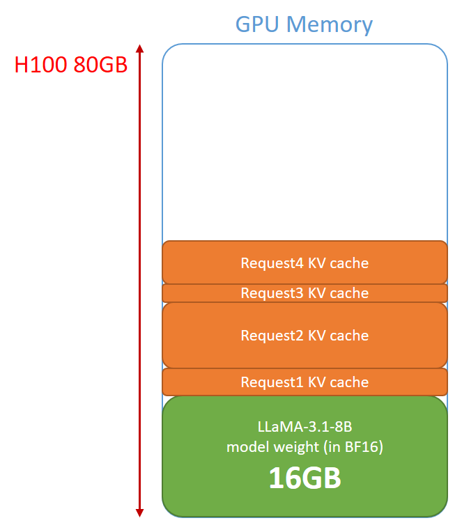
image: GPU Memory 示意圖

因此我們在 GPU 最多可以放的 KV cache length (tokens) 可以由以下公式來表示：

Press enter or click to view image in full size

而 KV cache 的大小我們又很好預估，GPT-2 跟 LLaMA-3.1 都可以套用我們剛剛的公式，唯一的差別是 LLaMA 系列有使用 Group Query Attention，KV head 的數量會比 Attention head 還要更少。

Press enter or click to view image in full size

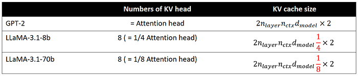
Table: KV cache size by models

同樣的算法甚至可以擴充到包含 Sliding window attention, Linear Attenion, …，就是後面的算式更複雜而已。

接下來我們帶入 H100-80GB 的 GPU Memory = 80GB，並且算 LLaMA-3.1 8b, 70b 在 bf16, fp8 precision 時，就可以得到下表。

Press enter or click to view image in full size

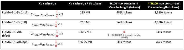
H100 80GB 上不同模型 setting 的 max concurrent KV cache length

可以看到單張 H100–80GB 的時候，LLaMA-3.1–8b (bf16) 能放 549k tokens，也就是說如果平均每個 user 使用 4k tokens 的 KV cache，那我們 GPU Memory 大約可以承受 137 個 concurrent users。但如果每個 user 平均使用 128k tokens 的 KV cache，就只能承受 4 個 concurrent users。

而單張 H100-80GB 則完全不能承受 LLaMA-3.1 70b (bf16)，必須將 H100 本身 quantize 成 fp8，並且如果也對 KV cache 做對應的 quantize，則可以勉強承受 30k tokens 的 KV cache。

這邊可以看到在 community 上常說的：「預估 GPU 大小大約要 = 1.2 * Model weight size 雖說有一定道理」，但嚴謹來看跟亂算沒有兩樣👿，因為沒辦法考慮不同使用場景（context 多長），也沒辦法討論不同 concurrent requests 的情況。

忽視這些基礎變因，則永遠無法做出正確的判斷

而如果遇到 GPU Memory 放完 model weight 還有餘裕但是目前被其他 request 的 KV cache 塞滿的情況時，正確來說我們就需要把其他沒有正在運算的 requests 的 KV cache offload 到 CPU Memory，像是 vllm 就有 --kv-transfer-config 這個參數，可以把優先度較低的 KV cache offload 到 CPU 上。

同時我們也需要把現在當筆 requests 的 KVcache 從 CPU Memory reload 回 GPU Memory（假設過去曾被 offload）。

因此我們總共需要 2 * KV_cache_size 的搬運來解決 GPU Memory 被其他 KV cache 塞滿的情況。

而這個搬運的效率則跟 GPU-CPU IO bandwidth 有關，通常都是走 PCIe，像 H100 預設是 PCIe Gen5 128GB/s。

因此我們發送一個 completion request 的時候，很大概率還要再等一個 offload/reload KV cache 的 latency，我們稱為 context switching latency。

Press enter or click to view image in full size

image: theoretical context switching latency

⭐ LLM theoretical inference latency 總結

在我們發送一個 request 時我們先後需要先等 context switching，進行 offload/reload KV cache，接下來我們需要 prefill 這次的 input prompt，接下來再進行 decoding。

其中每一個部分我們都有了一個分析框架，而這些分析框架其實都不是新東西，在過去分析 CNN edge computing 就很常用。

在 2024 年 Yao Fu 大神 [6] 也整理了一次 LLM 的分析框架，LLM Viewer 的作者在更早也提出了非常相似的框架 [4]，筆者本篇其實並沒有比他們多整理甚麼，更多是對一些基礎知識的補充說明，幫助大家更好串聯整體知識。

Press enter or click to view image in full size

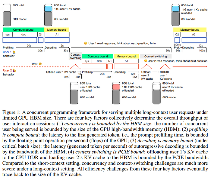
image from [6]: 其實已經完美的分析了 LLM inference latency，本篇更多只是做為一個補充說明。

實際上這篇論文也是筆者回去帶實驗室新生的必讀論文，不論是不是要做 LLM inference 相關，具體了解 inference 的過程幫助還是很大。

3. 結合現實考量: MFU 與 MBU

前面藉由 GPU 的 datasheet, LLM inference 的具體運算以及 roofline model 來討論理論數據，接下來我們要更近一步討論怎麼樣用理論來理解現實情況。

如何用理論映照現實，關鍵就是兩個問題：

理論數據跟實際數據在哪些情況下可以呈現高度相關性？
如何建立一個理論與實際情況的關係？

在年初 DeepSeek 爆紅的時候，筆者曾寫過一篇文章分析 DeepSeek V3 的訓練成本到底合不合理（結論是合理 XD）

[

【LLM 專欄】Deepseek v3 的訓練時間到底合不合理？淺談 LLM Training efficiency

判斷 2025 年企業到底要不要跟風投入打造各自的 deepseek v3

axk51013.medium.com

](https://axk51013.medium.com/deepseek-v3-%E7%9A%84%E8%A8%93%E7%B7%B4%E6%99%82%E9%96%93%E5%88%B0%E5%BA%95%E5%90%88%E4%B8%8D%E5%90%88%E7%90%86-%E6%B7%BA%E8%AB%87-llm-training-6460374b6d0f?source=post_page—–32164c253627—————————————)

其中就引入了 MFU （Model FLOPs Utilization）這個指標，藉由實際情況跟理論情況的比例，來判斷是否合理。

image: MFU 計算方法

在討論 DeepSeek V3 時，筆者藉由觀察其他主流的框架、專案、研究在 training LLM 的經驗，畫出了一個合理的 MFU 區間。

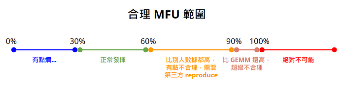
image: 合理 MFU 範圍

現在我們也要對 inference 做同樣的事情，利用前文我們分析的 LLM inference theoretical latency 資訊，以及其他專案的經驗來判斷實際情況。

在開始分析前我們必須了解，前文提到 Prefilling 大部分情況都是 GPU Computation Bound，而 Decoding 則大部分情況都是 GPU Memory Bandwidth Bound，因此分析 Prefilling 時我們可以套用 MFU，討論運算效率的比例，而分析 Decoding 實則需要套用 MBU（Model Bandwidth Utilization）

Press enter or click to view image in full size

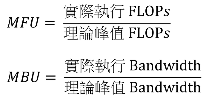
MFU vs MBU

1️⃣ 理論數據跟實際數據在哪些情況下可以呈現高度相關性？

首先需要解決的第一個問題是 MFU 跟 MBU 到底有沒有效？理論情況跟實際情況是否可以常態呈現某種固定比例？

這個問題 IBM 的團隊做過非常簡單的分析 [7]，他們建立 ML 模型來預測不同 LLM 實際在 vllm 跟 triton 的 inference 效率。

其中他們實測了兩種 feature set

把 model config 直接丟給 ML model 做預測，像是模型參數、vocabulary size、hidden size、…等
把 roofline model 分析結果丟給 ML model 做預測，也就是我們前文的分析方法後續再丟給 ML model。

而當提供 roofline model 的數據時，利用理論數據預測實際情況的精準度就達到 R^2 = 0.97+，已經是非常精準的預測結果，也顯現出遠比直接提供 model config 還要更準。

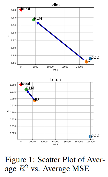
image from [7]，RLM 代表的是 roofline model, 而 ID 跟 OOD 都是使用 model config 丟給 ML model 做預測，ID 代表 in distribution, OOD 代表 out of distribution

從上述實驗我們可以得知實際 vllm/triton inference 情況跟理論 roofline 預測具備某種「線性關係」，因此 MFU 跟 MBU 是可用的。

實際情況其實還需要嚴謹的把不同 concurrent, token batch 拉出來談，IBM 這篇論文其實實驗做的算很隨便，不過筆者自己 reproduce 在 4090, A100, H100 也可以得出相似結論。

2️⃣ 如何建立一個理論與實際情況的關係？

已知 MFU 跟 MBU 具有一定的效果，那剩下的問題就很簡單了，統計各種第三方數據來了解 inference 時的 MFU 跟 MBU 數據應當為多少。

Prefilling MFU 統計：

Google 用 64 TPU v4 來 Prefill PaLM 540B，正常情況可以達成 30~40% MFU，而 Large Batch 可以得到 76%。[8]
Microsoft 的團隊在 H100 上面以不同的 parallelism 來跑 LLaMA-3 70B，普遍可以得到 30~40% 之間 MFU，最佳結果可以得到 ~70%。[9]
DynaServe 的團隊在 A100 上面測試不同 serve LLM 的方式，在 prefilling 為主的階段也都可以得到 ~40% 左右的 MFU。[10]

因此我們可以得到一個結論，在 Prefilling 時，MFU 正常情況在 30~40%，當 batchsize 提升或是有做比較深入的優化後，有機會達到 70~80% 之間。

實際上因應 vllm 的 default 設定很大概率不會最適應我們手上專案的場景，所以 MFU 通常會比 30% 還要顯著更低，大多時候如果未經系統化的調整，大多我聽到的國內企業內 inference service 即便在 peak usage 時 MFU 都在 ~5% 上下。

Decoding MBU 統計

MBU 因為是一個較新比較非正式的公式，因此討論的人比較少，我們就重點關注 DataBrick 的 blog <LLM Inference Performance Engineering: Best Practices>，其中統計的 MBU。

Press enter or click to view image in full size

image from [12]，可以看到 batchsize 較高時 MBU 會略為下降，而 GPU 多卡時 MBU 也會再下降，主要因素包含 interGPU communication，也包含多 GPU parallel 下，非運算/IO相關操作的占比會比較高。

Press enter or click to view image in full size

image from [12]，多卡時 MBU 大多都會再降低

可以看到 MBU 在不同 setting 下，大約在 25~66% 間搖擺，所以我們一般可以用 1/4~1/2 來當作標準。

我們也可以把第三方測試數據拿進來做運算，舉例而言極客灣去年年底評測過 M4 Pro, M4 Max 上 host Qwen2.5 不同大小的的 decoding latency (tokens/s)。

Press enter or click to view image in full size

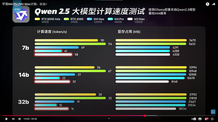
極客灣評測 Qwen2.5 在不同硬體，尤其是 M4 上的效率 https://youtu.be/2jEdpCMD5E8?t=840，注意這是 quantize 到 int4 的數字，每一個 parameter 只佔 0.5 Byte。

如果我們把數字帶入我們前文的公式，可以算出不論哪個硬體、哪個大小的模型，大約都是 40~50% 的 MBU（大概是因為極客灣在測試時都是單 GPU 測試）。

從上述我們可以知道三個基本結論

利用 roofline model 來估算的 MFU, MBU 確實有效
MFU 的正常區間在 30%~70%。
MBU 的正常區間在 25%~50%。

並且實務上我們可以很輕鬆的利用這組數字來估算在特定 GPU 設置、Model config 底下，我們可以預期得到的 Prefilling 跟 Decoding Latency 分別會是多少。

並更進一步基於我們的具體需求去調整我們的硬體配置、軟體優化方案。

結論

本文希望帶大家看懂 LLM inference 時到底發生甚麼事情，並且基於對基礎知識的詳細了解，建立出 LLM inference 的分析框架。

先後筆者講解了幾個關鍵概念

LLM 一次正向傳導（Forward Pass）具體發生了甚麼
LLM 一次 completion 的完整運算
Arithmetic Intensity 跟 Roofline model
以及基於以上理論分析以及 MFU/MBU 來看實際 inference latency

實際上本文的分析框架對於 LLM inference acceleration 相關議題，只是基礎中的基礎，但對於未來很多筆者想討論的題目而言，又是不可或缺的關鍵知識，因此特別撰寫這一篇，來為未來的更深入議題鋪墊。

不過只要看懂這篇，我們就可以對很多硬體 spec 有更敏感的判斷，舉例而言，最近 Nvidia 跟 Mediatek 合推的 DGX Spark 個人 AI Server，在官方宣傳上宣稱可以輕鬆 host 200B models。

Press enter or click to view image in full size

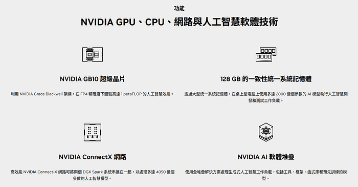
https://www.nvidia.com/zh-tw/products/workstations/dgx-spark/ 宣稱可以 host 200B 參數模型

但如果我們仔細看他的 spec（下圖），就會發現首先 System Memory 是 128GB 的 share memory，也就是說 200B model 也需要 quantize 成 int4 或是 fp4 才放得下，如果要放滿血板就要做逐層的 offloading。

Press enter or click to view image in full size

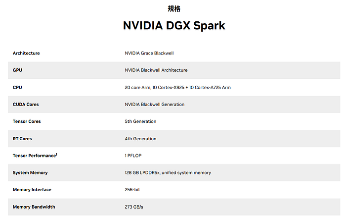
https://www.nvidia.com/zh-tw/products/workstations/dgx-spark/ DGX Spark 的具體 spec

同時即便真的放了 200B model FP4，因為 Bandwidth 只有 273 GB/s，考量到 MBU 大約 50%，我們也只能得到約 1 token/sec，也就是說離我們現在基本要求 30~50 tokens/sec 還有一大段距離。

因此如果購買 DGX Spark ，更正確的使用方法應該是以下三種

可以容忍 High Latency 的 inference 場景，ex: 一些任務用 O3, Claude4 跑 20 分鐘，同時可能要消耗幾十美元，我們用 DGX Spark + 大模型，可能可以用一個晚上跑出一樣效果，用時間換成本（DGX Spark 的用電很低，因此大概會划算）
Large Batch inference，雖然 bandwidth 很差，但 computation 還行，因此我們可以把 batchsize 拉大，像是 Test time search, parallel sampling，盡量往 roofline model 的右側去走。
Small Scale Finetuning，我們也可以乾脆就走 finetuning，但因為總運算量也沒非常大，所以大概率還是針對小模型或是 LoRA 的場景。

如果熟悉 LLM inference 就可以很輕鬆的建立這種對 GPU 配置的理解，並針對自己所需場景做 cp 值最高的安排。

Reference

Nvidia Accelerating a Hugging Face Llama 2 and Llama 3 models with Transformer Engine document https://docs.nvidia.com/deeplearning/transformer-engine/user-guide/examples/te_llama/tutorial_accelerate_hf_llama_with_te.html
Kaplan, Jared, et al. “Scaling laws for neural language models.” arXiv preprint arXiv:2001.08361 (2020).
Gu, Albert, and Tri Dao. “Mamba: Linear-time sequence modeling with selective state spaces.” arXiv preprint arXiv:2312.00752 (2023).
Yuan, Zhihang, et al. “Llm inference unveiled: Survey and roofline model insights.” arXiv preprint arXiv:2402.16363 (2024).
DeepMind How to Scale Your Model Part7 All About Transformer Inference
Fu, Yao. “Challenges in deploying long-context transformers: A theoretical peak performance analysis.” arXiv preprint arXiv:2405.08944 (2024).
Imai, Saki, et al. “Predicting LLM Inference Latency: A Roofline-Driven ML Method.” Annual Conference on Neural Information Processing Systems. 2024.
Pope, Reiner, et al. “Efficiently scaling transformer inference.” Proceedings of machine learning and systems 5 (2023): 606–624.
Agrawal, Amey, et al. “Medha: Efficiently Serving Multi-Million Context Length LLM Inference Requests Without Approximations.” arXiv preprint arXiv:2409.17264 (2024).
Ruan, Chaoyi, et al. “DynaServe: Unified and Elastic Execution for Dynamic Disaggregated LLM Serving.” arXiv preprint arXiv:2504.09285 (2025).
Optimizing vLLM Performance on A100 80GB: Benchmark Insights and Recommendations https://www.databasemart.com/blog/vllm-gpu-benchmark-a100-80gb?srsltid=AfmBOooF4Npy5eI7yMFCD2-iOkbCbqvlfIANGUMl9VrutipmIjOItvbd

DataBrick

LLM Inference Performance Engineering: Best Practices https://www.databricks.com/blog/llm-inference-performance-engineering-best-practices?utm_source=chatgpt.com

[

Large Language Models

](https://medium.com/tag/large-language-models?source=post_page—–32164c253627—————————————)

[

Llm

](https://medium.com/tag/llm?source=post_page—–32164c253627—————————————)

[

](https://medium.com/tag/ai?source=post_page—–32164c253627—————————————)

[

Genai

](https://medium.com/tag/genai?source=post_page—–32164c253627—————————————)

[

Transformers

](https://medium.com/tag/transformers?source=post_page—–32164c253627—————————————)

165

[

](https://axk51013.medium.com/?source=post_page—post_author_info–32164c253627—————————————)

[

Written by 倢愷 Oscar

](https://axk51013.medium.com/?source=post_page—post_author_info–32164c253627—————————————)

2.3K followers

·85 following

我是倢愷，CTO at TeraThinker an AI Adaptive Learning System Company。AI/HCI研究者，超過100場的ML、DL演講、workshop經驗。主要學習如何將AI落地於業界。有家教、演講合作，可以email跟我聯絡：axk51013@gmail.com

No responses yet

Write a response

[

What are your thoughts?

](https://medium.com/m/signin?operation=register&redirect=https%3A%2F%2Faxk51013.medium.com%2Fllm-%25E5%25B0%2588%25E6%25AC%2584-%25E8%25A9%25B3%25E8%25A7%25A3-llm-inference-efficiency-32164c253627&source=—post_responses–32164c253627———————respond_sidebar——————)

Cancel

Respond

More from 倢愷 Oscar

[

](https://axk51013.medium.com/?source=post_page—author_recirc–32164c253627—-0———————8b0bb5f4_3030_4305_8c8b_c585eb586374————–)

[

倢愷 Oscar

](https://axk51013.medium.com/?source=post_page—author_recirc–32164c253627—-0———————8b0bb5f4_3030_4305_8c8b_c585eb586374————–)

[

【LLM專欄】All about Lora

LLM最重要技術之一，一篇文章深入淺出Lora的方方面面

](https://axk51013.medium.com/llm%E5%B0%88%E6%AC%84-all-about-lora-5bc7e447c234?source=post_page—author_recirc–32164c253627—-0———————8b0bb5f4_3030_4305_8c8b_c585eb586374————–)

Jun 2, 2024

[

451

[

](https://axk51013.medium.com/?source=post_page—author_recirc–32164c253627—-1———————8b0bb5f4_3030_4305_8c8b_c585eb586374————–)

[

倢愷 Oscar

](https://axk51013.medium.com/?source=post_page—author_recirc–32164c253627—-1———————8b0bb5f4_3030_4305_8c8b_c585eb586374————–)

[

不要再用K-means！超實用分群法DBSCAN詳解

sklearn DBSCAN使用介紹

](https://axk51013.medium.com/%E4%B8%8D%E8%A6%81%E5%86%8D%E7%94%A8k-means-%E8%B6%85%E5%AF%A6%E7%94%A8%E5%88%86%E7%BE%A4%E6%B3%95dbscan%E8%A9%B3%E8%A7%A3-a33fa287c0e?source=post_page—author_recirc–32164c253627—-1———————8b0bb5f4_3030_4305_8c8b_c585eb586374————–)

Apr 7, 2021

[

900

[

](https://axk51013.medium.com/?source=post_page—author_recirc–32164c253627—-2———————8b0bb5f4_3030_4305_8c8b_c585eb586374————–)

[

倢愷 Oscar

](https://axk51013.medium.com/?source=post_page—author_recirc–32164c253627—-2———————8b0bb5f4_3030_4305_8c8b_c585eb586374————–)

[

【LLM 10大觀念-3】快速建造自己個instruction tuning dataset

迎接2024年：10個必須要搞懂的LLM概念-3

](https://axk51013.medium.com/llm-10%E5%A4%A7%E8%A7%80%E5%BF%B5-3-%E5%BF%AB%E9%80%9F%E5%BB%BA%E9%80%A0%E8%87%AA%E5%B7%B1%E5%80%8Binstruction-tuning-dataset-ab391eba61e5?source=post_page—author_recirc–32164c253627—-2———————8b0bb5f4_3030_4305_8c8b_c585eb586374————–)

Apr 20, 2024

[

250

[

](https://axk51013.medium.com/?source=post_page—author_recirc–32164c253627—-3———————8b0bb5f4_3030_4305_8c8b_c585eb586374————–)

[

倢愷 Oscar

](https://axk51013.medium.com/?source=post_page—author_recirc–32164c253627—-3———————8b0bb5f4_3030_4305_8c8b_c585eb586374————–)

[

不要再做One Hot Encoding！！

Categorical feature的正確開啟方式

](https://axk51013.medium.com/%E4%B8%8D%E8%A6%81%E5%86%8D%E5%81%9Aone-hot-encoding-b5126d3f8a63?source=post_page—author_recirc–32164c253627—-3———————8b0bb5f4_3030_4305_8c8b_c585eb586374————–)

Apr 15, 2021

[

1.5K

[

See all from 倢愷 Oscar

](https://axk51013.medium.com/?source=post_page—author_recirc–32164c253627—————————————)

Recommended from Medium

[

](https://medium.com/@sonitanishk2003?source=post_page—read_next_recirc–32164c253627—-0———————09323d73_568f_4879_8f7a_20e6820725ba————–)

[

Tanishk Soni

](https://medium.com/@sonitanishk2003?source=post_page—read_next_recirc–32164c253627—-0———————09323d73_568f_4879_8f7a_20e6820725ba————–)

[

The Ultimate Guide to LLM Memory: From Context Windows to Advanced Agent Memory Systems

A Deep-Dive into Theory, Code, and a Hands-on Project to Master Context Management in AI

](https://medium.com/@sonitanishk2003/the-ultimate-guide-to-llm-memory-from-context-windows-to-advanced-agent-memory-systems-3ec106d2a345?source=post_page—read_next_recirc–32164c253627—-0———————09323d73_568f_4879_8f7a_20e6820725ba————–)

Jul 19

[

](https://pub.towardsai.net/?source=post_page—read_next_recirc–32164c253627—-1———————09323d73_568f_4879_8f7a_20e6820725ba————–)

[

Towards AI

](https://pub.towardsai.net/?source=post_page—read_next_recirc–32164c253627—-1———————09323d73_568f_4879_8f7a_20e6820725ba————–)

[

Alpha Iterations

](https://medium.com/@alphaiterations?source=post_page—read_next_recirc–32164c253627—-1———————09323d73_568f_4879_8f7a_20e6820725ba————–)

[

Building an AI Agent with Model Context Protocol (MCP): A Complete Guide

From theory to practice: Learn how Model Context Protocol (MCP) solves AI integration challenges while building a weather and search agent…

](https://medium.com/@alphaiterations/building-an-ai-agent-with-model-context-protocol-mcp-a-complete-guide-37b8f6cd7b2b?source=post_page—read_next_recirc–32164c253627—-1———————09323d73_568f_4879_8f7a_20e6820725ba————–)

Nov 16

[

117

[

](https://iotforce.medium.com/?source=post_page—read_next_recirc–32164c253627—-0———————09323d73_568f_4879_8f7a_20e6820725ba————–)

[

Kruk Matias

](https://iotforce.medium.com/?source=post_page—read_next_recirc–32164c253627—-0———————09323d73_568f_4879_8f7a_20e6820725ba————–)

[

Scaling AI Agents with DSPy and MIPROv2: From Manual Prompts to Automated Optimization

Part 5 of 7. ← Part 4: Auditability • ← Part 3: Not all shining is gold • ← Part 2: Multi-Role Pipeline • Part 1: The Vision

](https://iotforce.medium.com/scaling-ai-agents-with-dspy-and-miprov2-from-manual-prompts-to-automated-optimization-6a88f993f2b2?source=post_page—read_next_recirc–32164c253627—-0———————09323d73_568f_4879_8f7a_20e6820725ba————–)

4d ago

[

](https://aakashgupta.medium.com/?source=post_page—read_next_recirc–32164c253627—-1———————09323d73_568f_4879_8f7a_20e6820725ba————–)

[

Aakash Gupta

](https://aakashgupta.medium.com/?source=post_page—read_next_recirc–32164c253627—-1———————09323d73_568f_4879_8f7a_20e6820725ba————–)

[

Google Just Dropped 70 Pages on Context Engineering. Here’s What Actually Matters.

Imagine an AI that remembers you’re vegan. Knows your debugging style. Recalls that project from three months ago without you repeating…

](https://aakashgupta.medium.com/google-just-dropped-70-pages-on-context-engineering-heres-what-actually-matters-c0df8d8e82cc?source=post_page—read_next_recirc–32164c253627—-1———————09323d73_568f_4879_8f7a_20e6820725ba————–)

Nov 15

[

713

[

](https://levelup.gitconnected.com/?source=post_page—read_next_recirc–32164c253627—-2———————09323d73_568f_4879_8f7a_20e6820725ba————–)

[

Level Up Coding

](https://levelup.gitconnected.com/?source=post_page—read_next_recirc–32164c253627—-2———————09323d73_568f_4879_8f7a_20e6820725ba————–)

[

Fareed Khan

](https://medium.com/@fareedkhandev?source=post_page—read_next_recirc–32164c253627—-2———————09323d73_568f_4879_8f7a_20e6820725ba————–)

[

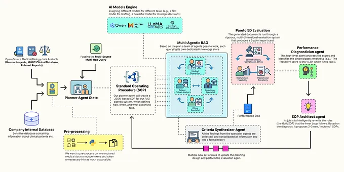
Building a Self-Improving Agentic RAG System

Specialist agents, multi-dimensional eval, Pareto front and more.

](https://medium.com/@fareedkhandev/building-a-self-improving-agentic-rag-system-f55003af44c4?source=post_page—read_next_recirc–32164c253627—-2———————09323d73_568f_4879_8f7a_20e6820725ba————–)

Nov 15

[

1.2K

[

](https://medium.com/data-science-collective?source=post_page—read_next_recirc–32164c253627—-3———————09323d73_568f_4879_8f7a_20e6820725ba————–)

[

Data Science Collective

](https://medium.com/data-science-collective?source=post_page—read_next_recirc–32164c253627—-3———————09323d73_568f_4879_8f7a_20e6820725ba————–)

[

Han HELOIR YAN, Ph.D. ☕️

](https://medium.com/@han.heloir?source=post_page—read_next_recirc–32164c253627—-3———————09323d73_568f_4879_8f7a_20e6820725ba————–)

[

Tiny Brains, Big Impact: How Small Language Models Are Redefining AI in the Real World

From transformer basics to real-world deployment — without the PhD

](https://medium.com/@han.heloir/tiny-brains-big-impact-how-small-language-models-are-redefining-ai-in-the-real-world-9ff66d8ea5ce?source=post_page—read_next_recirc–32164c253627—-3———————09323d73_568f_4879_8f7a_20e6820725ba————–)

Nov 16

[

803

[

See more recommendations

](https://medium.com/?source=post_page—read_next_recirc–32164c253627—————————————)

[

Help

](https://help.medium.com/hc/en-us?source=post_page—–32164c253627—————————————)

[

Status

](https://status.medium.com/?source=post_page—–32164c253627—————————————)

[

About

](https://medium.com/about?autoplay=1&source=post_page—–32164c253627—————————————)

[

Careers

](https://medium.com/jobs-at-medium/work-at-medium-959d1a85284e?source=post_page—–32164c253627—————————————)

[

Press

](mailto:pressinquiries@medium.com)

[

Blog

](https://blog.medium.com/?source=post_page—–32164c253627—————————————)

[

Privacy

](https://policy.medium.com/medium-privacy-policy-f03bf92035c9?source=post_page—–32164c253627—————————————)

[

Rules

](https://policy.medium.com/medium-rules-30e5502c4eb4?source=post_page—–32164c253627—————————————)

[

Terms

](https://policy.medium.com/medium-terms-of-service-9db0094a1e0f?source=post_page—–32164c253627—————————————)

[

Text to speech

](https://speechify.com/medium?source=post_page—–32164c253627—————————————)

You are signed out. Sign in with your member account (al__@g__.com) to view other member-only stories. Sign in

Source

【LLM 專欄】詳解 LLM inference efficiency

我們需要多少 GPU 來建立穩定的 LLM 服務？

0. Preliminary: LLM inference 的時候到底發生了甚麼事情

⭐ Part2: LLM completion 過程：Prefilling vs Decoding

1. 評斷 LLM 的運算效率 Roofline Model and Arithmetic Intensity

Get 倢愷 Oscar’s stories in your inbox

2. LLM inference Latency 估計

3. 結合現實考量: MFU 與 MBU

【LLM 專欄】Deepseek v3 的訓練時間到底合不合理？淺談 LLM Training efficiency

判斷 2025 年企業到底要不要跟風投入打造各自的 deepseek v3

結論

Reference

Written by 倢愷 Oscar

No responses yet

More from 倢愷 Oscar

【LLM專欄】All about Lora

LLM最重要技術之一，一篇文章深入淺出Lora的方方面面

不要再用K-means！ 超實用分群法DBSCAN詳解

sklearn DBSCAN使用介紹

【LLM 10大觀念-3】快速建造自己個instruction tuning dataset

迎接2024年：10個必須要搞懂的LLM概念-3

不要再做One Hot Encoding！！

Categorical feature的正確開啟方式

Recommended from Medium

The Ultimate Guide to LLM Memory: From Context Windows to Advanced Agent Memory Systems

A Deep-Dive into Theory, Code, and a Hands-on Project to Master Context Management in AI

Building an AI Agent with Model Context Protocol (MCP): A Complete Guide

From theory to practice: Learn how Model Context Protocol (MCP) solves AI integration challenges while building a weather and search agent…

Scaling AI Agents with DSPy and MIPROv2: From Manual Prompts to Automated Optimization

Part 5 of 7. ← Part 4: Auditability • ← Part 3: Not all shining is gold • ← Part 2: Multi-Role Pipeline • Part 1: The Vision

Google Just Dropped 70 Pages on Context Engineering. Here’s What Actually Matters.

Imagine an AI that remembers you’re vegan. Knows your debugging style. Recalls that project from three months ago without you repeating…

Building a Self-Improving Agentic RAG System

Specialist agents, multi-dimensional eval, Pareto front and more.

Tiny Brains, Big Impact: How Small Language Models Are Redefining AI in the Real World

From transformer basics to real-world deployment — without the PhD

不要再用K-means！超實用分群法DBSCAN詳解