Reference
(1) Geometric Calculus 1 - YouTube : 4 lectures series, very good.
Stokes’ Theorem on Manifolds (youtube.com) : 非常好的 lecture to combine vector calculus!
Takeaways
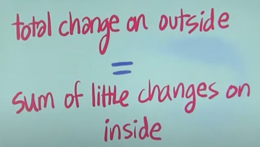
- 所有微積分可以歸納成一個基本原理:“total change on outside = sum of little changes on inside”
- 不要小看這句話,左邊代表 global property (全域特性,例如拓撲特徵,對稱性,奇點)。右邊代表 local property (局部特性/分析,例如斜率,梯度,旋度,散度,甚至曲率)
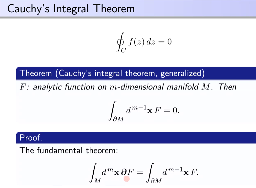
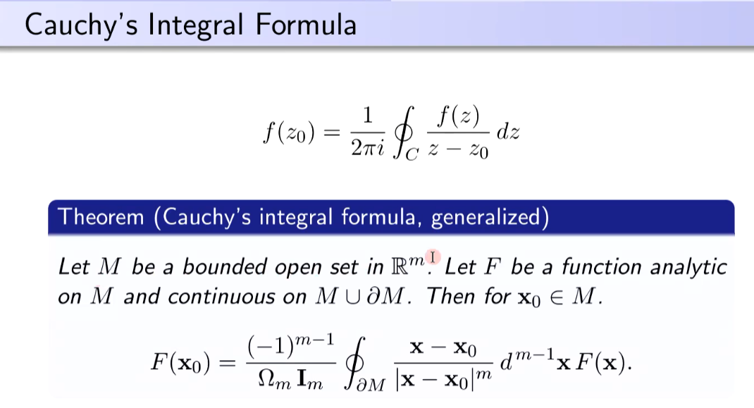
- 如果是有源 (source or sink),有兩種處理方式:(1) “total change on outside = sum of little changes on inside + source/sink generation rate”; (2) 加上新的邊界把 source/sink 變成 outside. Cauchy 就是這方面的高手 (複分析)。
Introduction
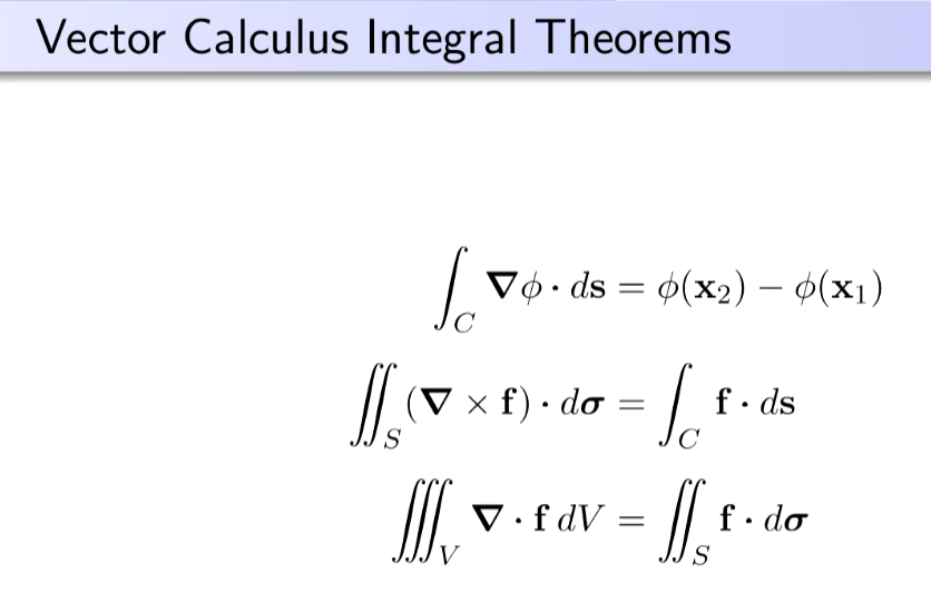
傳統的 Vector calculus 三大定理 (in 3D space):
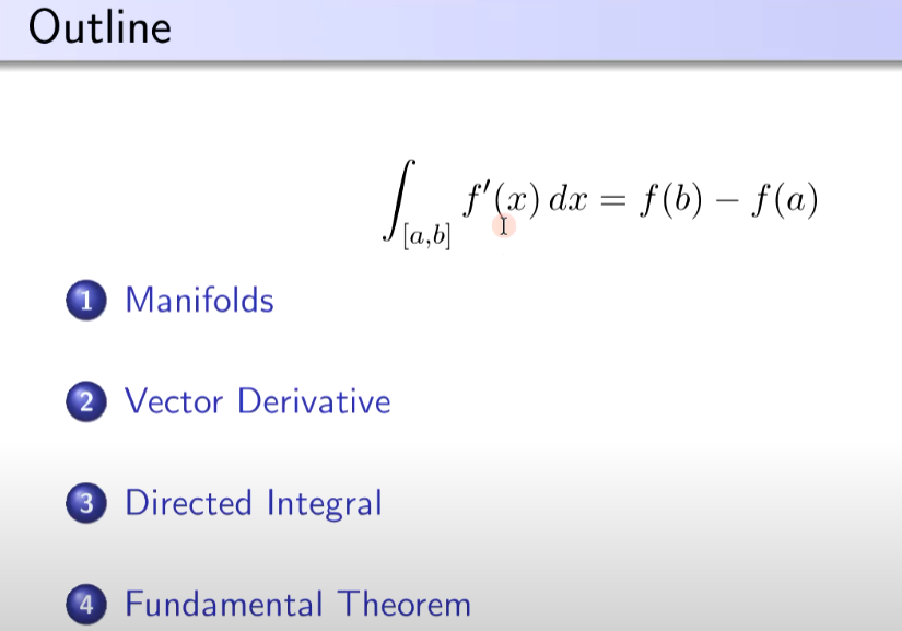
(Gradient Theorem) : $\int_a^b \nabla \varphi \cdot dl = \varphi(b) - \varphi(a)$
(Curl/Stokes Theorem) : $\iint_S \nabla \times \vec{A} \cdot ds = \oint_c \vec{A}\cdot dl$
(Divergence Theorem) : $\iiint_V \nabla \cdot \vec{A} \,dv = \iint_S \vec{A}\cdot ds$
三者看起來都像是某種形式的微積分定理:左邊是積分一個“微分形式的純量或向量函數”,等於右邊純量或向量函數 “少一階”在 boundary的積分。我們的挑戰是否能用一個定理整合三個定理?
- Gradient theorem 在 1D 空間簡化成牛頓的微積分定理。
- Gradient, Curl, Divergence 定理都有很清晰的物理意義。
- Gradient, Curl, Divergence 等 “微分”作用的純量和向量,似乎有機會用 Geometric Algebra 結合!
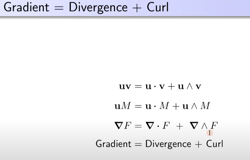
- Hint: $\nabla \vec{A} = \nabla \cdot \vec{A} + \nabla \wedge \vec{A} $
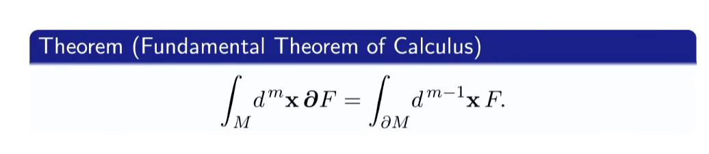
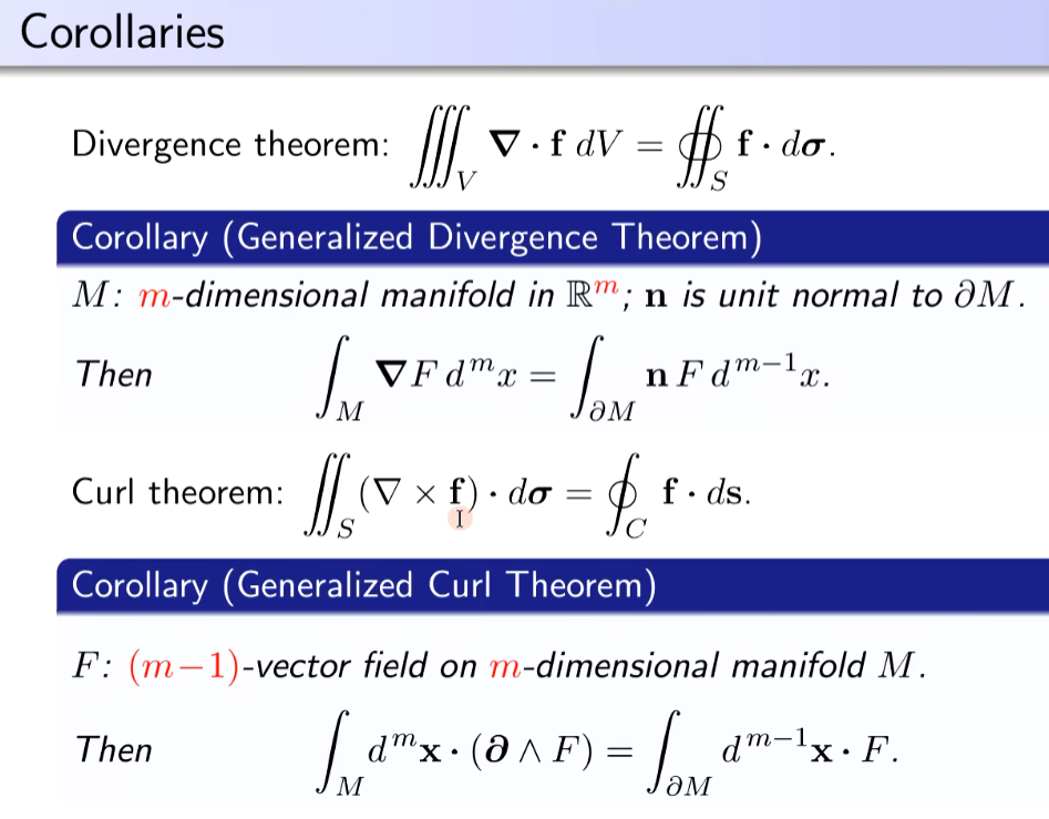
- 概念上形式: $\int \cdots \int_U \nabla\vec{A}\cdot dx^{n} = \int \cdots \int_{\partial U} \vec{A} \cdot dx^{n-1}$ 此處 $\partial U$ 是 $U$ 的 boundary.
但 GA Calculus 重點是
- 物理意義
- 有物理意義就容易得到和坐標系無關的形式
- 坐標系無關就容易推廣到曲面 (manifold) 的形式
- 比較 tensor calculus 和 Einstein symbol, covariant/contravariant form.
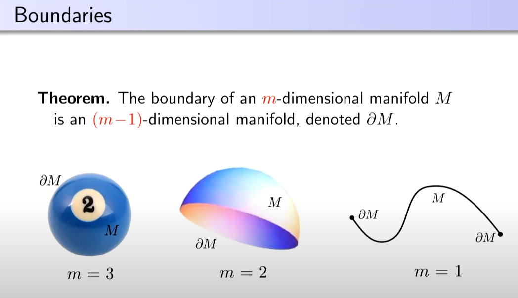
我們不限制在歐式空間,所以先定義 Manifold:
Manifold and Tangent (Vector) Space (定義和 GA 無關)
幾個重點
-
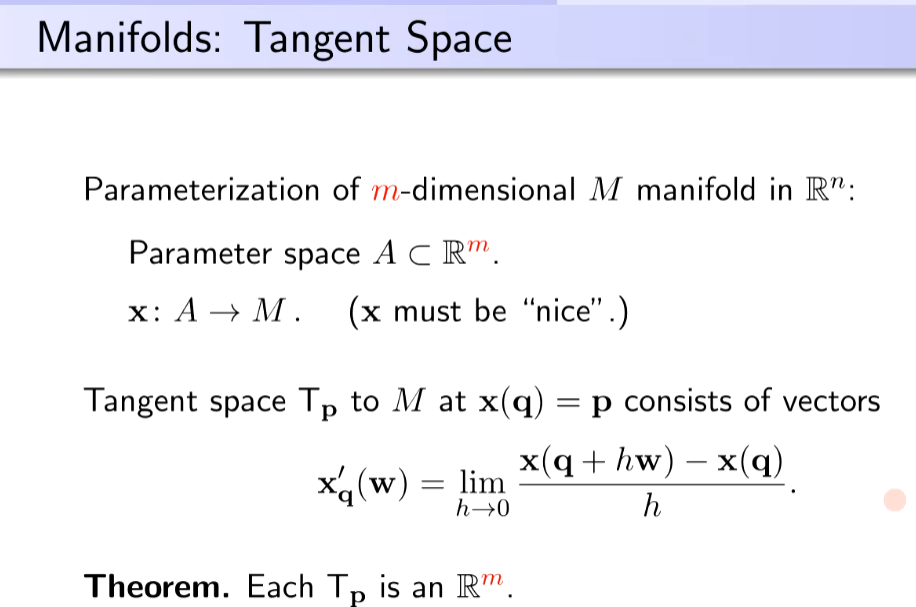
Parameterized manifold: $m$-dimensional $M$ manifold in $R^n$. Parameter space $A \subset R^m.$
$\mathbf{x}: A \to M$
-
Tangent space: $T_p$ to $M$ at $\mathbf{x}(q)= p$ 包含 vectors
$\mathbf{x}’q(w) = \lim{h\to 0} \frac{\mathbf{x}(q+hw)-\mathbf{x}(q)}{h}$
- 注意:Tangent space 的 dimension 和 manifold 相同 ($R^m$)
- 1D 的 tangent space 就是切向量 (tangent vector)
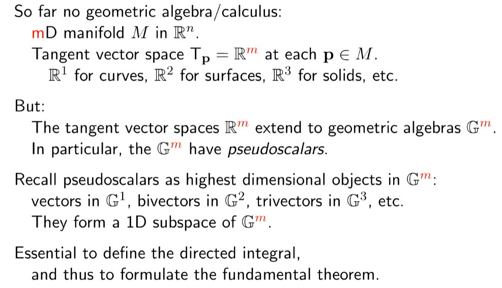
- Geometric Algebra 就是把 $T_p$ vector space $R^m$ extent to $G^m$
- $G^1$ 包含 scalar (1) and pseudo-scalar (1), 2-DOF (degree of freedom)
- $G^2$ 包含 scalar (1), vector (2), and bivector (pseudo-scalar) (1), 4-DOF
- $G^3$ 包含 scalar (1), vector (3), bivector (3), trivector (pseudo-scalar) (1), 8-DOF
- Pseudo-scalar forms a 1D subspace of $G^m$, 後面會用來定義 directed integral.

Vector Gradient
Gradient theorem 的 gradient 作用在純量函數,產生向量函數。
此處類似,不過把 basis vector ($e_1$, $e_2$) 放在微分項前面,而不是後面。
Q: 比較 tensor analysis 的 gradient!
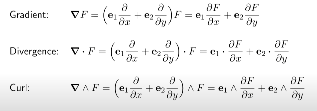
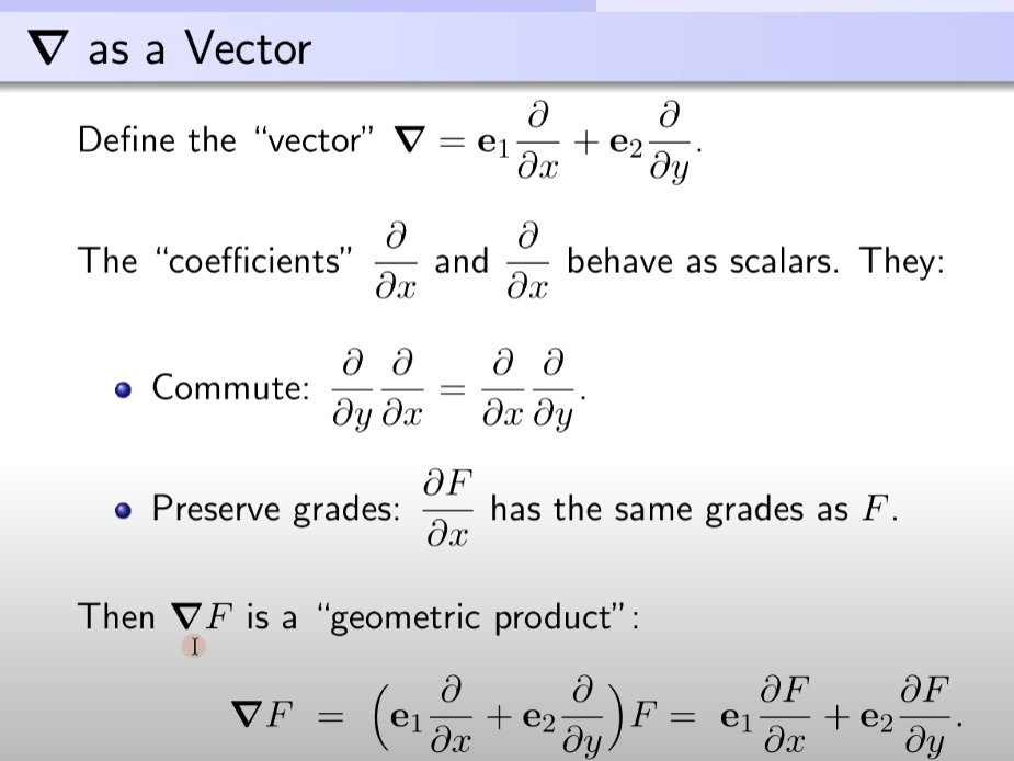
我們定義 $\nabla$ as a Vector : $\boldsymbol{\nabla}=\mathbf{e}_1 \frac{\partial}{\partial x}+\mathbf{e}_2 \frac{\partial}{\partial y}$. The “coefficients” $\frac{\partial}{\partial x}$ and $\frac{\partial}{\partial x}$ behave as scalars. They
- Commute: $\frac{\partial}{\partial y} \frac{\partial}{\partial x}=\frac{\partial}{\partial x} \frac{\partial}{\partial y}$.
- Preserve grades: $\frac{\partial F}{\partial x}$ has the same grades as $F$. Then $\boldsymbol{\nabla} F$ is a “geometric product”: \(\boldsymbol{\nabla} F=\left(\mathbf{e}_1 \frac{\partial}{\partial x}+\mathbf{e}_2 \frac{\partial}{\partial y}\right) F=\mathbf{e}_1 \frac{\partial F}{\partial x}+\mathbf{e}_2 \frac{\partial F}{\partial y} .\) Gradient: $\quad \boldsymbol{\nabla} F=\left(\mathbf{e}_1 \frac{\partial}{\partial x}+\mathbf{e}_2 \frac{\partial}{\partial y}\right) F=\mathbf{e}_1 \frac{\partial F}{\partial x}+\mathbf{e}_2 \frac{\partial F}{\partial y}$ Divergence: $\quad \boldsymbol{\nabla} \cdot F=\left(\mathbf{e}_1 \frac{\partial}{\partial x}+\mathbf{e}_2 \frac{\partial}{\partial y}\right) \cdot F=\mathbf{e}_1 \cdot \frac{\partial F}{\partial x}+\mathbf{e}_2 \cdot \frac{\partial F}{\partial y}$ Curl: $\quad \boldsymbol{\nabla} \wedge F=\left(\mathbf{e}_1 \frac{\partial}{\partial x}+\mathbf{e}_2 \frac{\partial}{\partial y}\right) \wedge F=\mathbf{e}_1 \wedge \frac{\partial F}{\partial x}+\mathbf{e}_2 \wedge \frac{\partial F}{\partial y}$ Gradient $=$ Divergence $+$ Curl \(\begin{aligned} \mathbf{u v} & =\mathbf{u} \cdot \mathbf{v}+\mathbf{u} \wedge \mathbf{v} \\ \mathbf{u} M & =\mathbf{u} \cdot M+\mathbf{u} \wedge M \\ \boldsymbol{\nabla} F & =\boldsymbol{\nabla} \cdot F+\boldsymbol{\nabla} \wedge F \\ \text { Gradient } & =\text { Divergence }+\text { Curl } \end{aligned}\)
Dual
Definition: Unit pseudo-scalar $ \mathbf{I} = \mathbf{e}_1 \mathbf{e}_2 \mathbf{e}_3$
Definition: Dual of a multivector $M$ is $M^* = M \mathbf{I}^{-1} = M \mathbf{e}_3 \mathbf{e}_2 \mathbf{e}_1$
Dual 之間的關係是通過 * 連接:
Theorem: Orthogonal complement
- Let blade $\mathbf{B}$ represent subspace $S$, then $\mathbf{B}^*$ represents the orthogonal complement of $S$. \(\begin{aligned}(M\wedge N)^* & = M \cdot N^* \\ (M\cdot N)^* & = M \wedge N^* \\(\mathbf{u} \wedge \mathbf{v})^* & = \mathbf{u} \times \mathbf{v} \end{aligned}\)
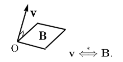
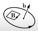
Dual theorem 用於 bivector. 以磁場爲例:(why negative? 左手?)
\(\begin{aligned} \mathbf{b} &: \text{magnetic field vector in 3D}\\
\mathbf{B} & = -\mathbf{b}^* = -\mathbf{b} \mathbf{I}^{-1} \end{aligned}\)
Maxwell Equation
Electric vector field: $\mathbf{e}$; Magnetic vector field: $\mathbf{b}$
Magnetic bivector field: $\mathbf{B}=-\mathbf{b}^*$, a bivector orthogonal to $\mathbf{b}$. \(\begin{array}{cccc} \boldsymbol{\nabla} \cdot \mathbf{e}=0 & \partial_t \mathbf{e}-\boldsymbol{\nabla} \times \mathbf{b}=0 & \partial_t \mathbf{b}+\boldsymbol{\nabla} \times \mathbf{e}=0 & \boldsymbol{\nabla} \cdot \mathbf{b}=0 \\ \boldsymbol{\nabla} \cdot \mathbf{e}=0 & \partial_t \mathbf{e}-(\boldsymbol{\nabla} \wedge \mathbf{b})^*=0 & \partial_t \mathbf{b}^*+(\boldsymbol{\nabla} \times \mathbf{e})^*=0 & \boldsymbol{\nabla} \wedge \mathbf{b}^*=0 \\ \boldsymbol{\nabla} \cdot \mathbf{e}=0 & \partial_t \mathbf{e}+\boldsymbol{\nabla} \cdot \mathbf{B}=0 & \partial_t \mathbf{B}+\boldsymbol{\nabla} \wedge \mathbf{e}=0 & \boldsymbol{\nabla} \wedge \mathbf{B}=0 \\ \boldsymbol{\nabla} \cdot \mathbf{e}=0 & \partial_t \mathbf{e}+\boldsymbol{\nabla} \cdot \mathbf{B}=0 & \partial_t \mathbf{B}+\boldsymbol{\nabla} \wedge \mathbf{e}=0 & \boldsymbol{\nabla} \wedge \mathbf{B}=0 \\ \text { scalar } & \text { vector } & \text { bivector } & \text { trivector } \\ & F=\mathbf{e}+\mathbf{B} . & \\ & \left(\partial_t+\boldsymbol{\nabla}\right) F=0 . \end{array}\) $F$ satisfies the wave equation: \(\begin{gathered} \left(\partial_t^2-\nabla^2\right) F=\left(\partial_t-\nabla\right)\left(\partial_t+\nabla\right) F \\ F=\mathbf{e}+\mathbf{B} \\ \left(\partial_t+\boldsymbol{\nabla}\right) F=0 \\ \mathbf{f}=q(\mathbf{e}-\mathbf{v} \cdot \mathbf{B}) \end{gathered}\)
Reciprocal Basis (同樣用於 Tensor Calculus)
Let ${\mathbf{b}_i}$ be a basis for ${\R}^n$. A unique reciprocal basis ${\mathbf{b}^i}$
$\mathbf{b}i \cdot \mathbf{b}^i = \delta{ij}$
Tangent Space Basis
Let $\mathbf{x}(u, v)$ parameterize a surface $S$, with $\mathbf{x}(u,v)=\mathbf{x}(\mathbf{q})=\mathbf{p}$ \(\mathbf{x}_u(\mathbf{q})=\frac{\partial \mathbf{x}(\mathbf{q})}{\partial u}=\lim _{h \rightarrow 0} \frac{\mathbf{x}\left(\mathbf{q}+h \mathbf{e}_u\right)-\mathbf{x}(\mathbf{q})}{h}=\mathbf{x}_{\mathbf{q}}^{\prime}\left(\mathbf{e}_u\right)\) Theorem (Tangent Space Basis) \(\left\{\mathbf{x}_u(\mathbf{q}), \mathbf{x}_v(\mathbf{q})\right\} \text { is a basis for } \mathrm{T}_{\mathbf{p}} \text {. }\)
Vector Derivative (和 Gradient 不同!!)
Vector calculus gradient: input scalar field, output vector field, 代表最陡峭的方向。original basis (u, v), NOT tangent space basis!
Geometric algebra (GA) calculus gradient: input vector field, output scalar (div) + vector (curl), 代表 ??
Vector calculus directional derivative (along u, for example): a scalar!
GA vector derivative: a vector (with 2 directional derivative multiply tangent space reciprocal basis?)
微分幾何永遠有兩套坐標系: global 坐標系 (u, v or e1, e2) 對應 parameter space basis, 這個坐標系和 manifold point P 無關。 Local 坐標系 (x_u, x_v) 對應 tangent space basis. 這個坐標系直接隨著 P 改變!!!
如何把 global coordinate and local coordinate 連接在一起: Levi-citi connection?? (point P and P+d 的 local 坐標系的關係)
| Input | Output | Basis | Meaning | |
|---|---|---|---|---|
| Gradient in VC | Scalar field | Vector field | u, v (or e1, e2) in parameter space (global coordinate) | steep descent最陡峭方向 |
| Gradient in GA | Vector field | div+curl (mixed scalar + vector field) | u, v (or e1, e2) in parameter space (global coordinate) | |
| Direction derivative in VC | Scalar field? | Scalar value at point P | Tangent space basis at P (local coordinate, vary with P) | Local derivative |
| Vector derivative in GA | Scalar field? | Vector (2 scalar values + directions) at point P | Tangent space basis at P (local coordinate, vary with P) | Local derivative |
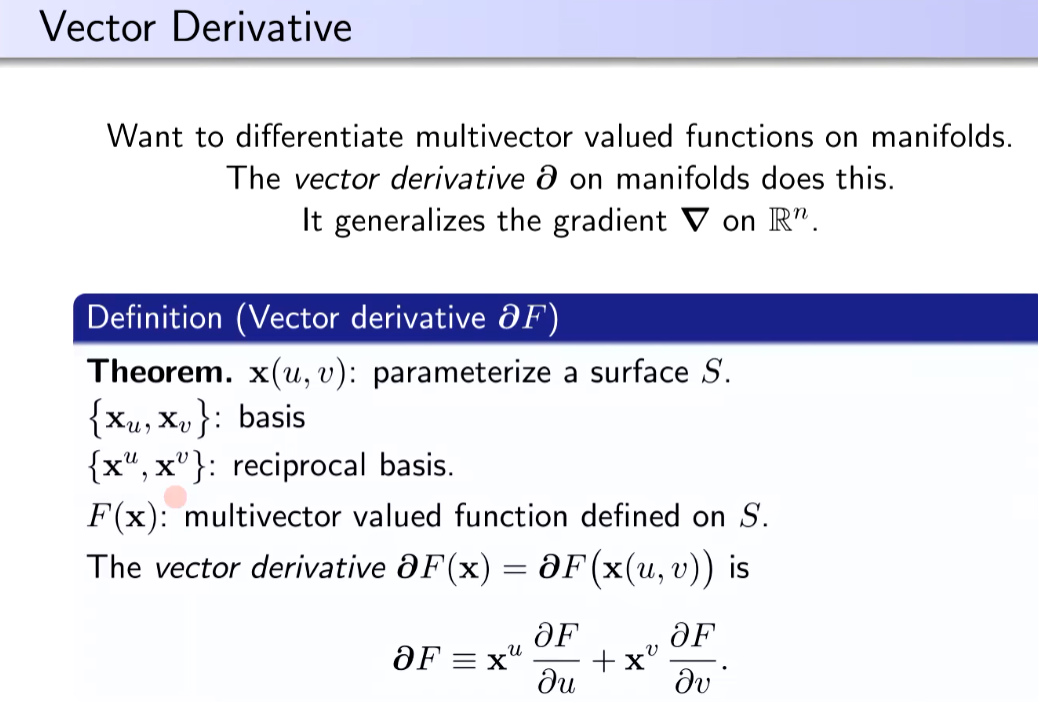
Theorem. $\mathbf{x}(u, v)$ : parameterize a surface $S$.
$\left{\mathbf{x}_u, \mathbf{x}_v\right}$ : basis
$\left{\mathbf{x}^u, \mathbf{x}^v\right}$ : reciprocal basis.
$F(\mathbf{x})$ : multivector valued function defined on $S$.
The vector derivative $\boldsymbol{\partial} F(\mathbf{x})=\boldsymbol{\partial} F(\mathbf{x}(u, v))$ is
\(\boldsymbol{\partial F} \equiv \mathbf{x}^u \frac{\partial F}{\partial u}+\mathbf{x}^v \frac{\partial F}{\partial v} \text {. }\)
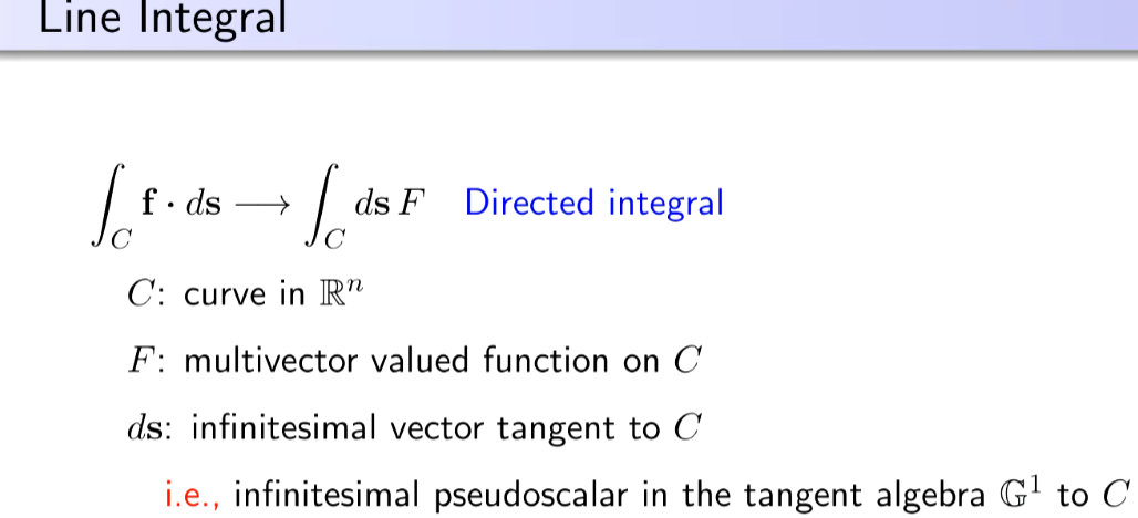
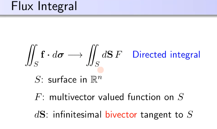
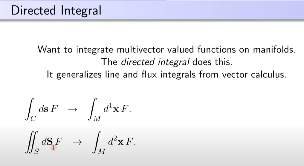
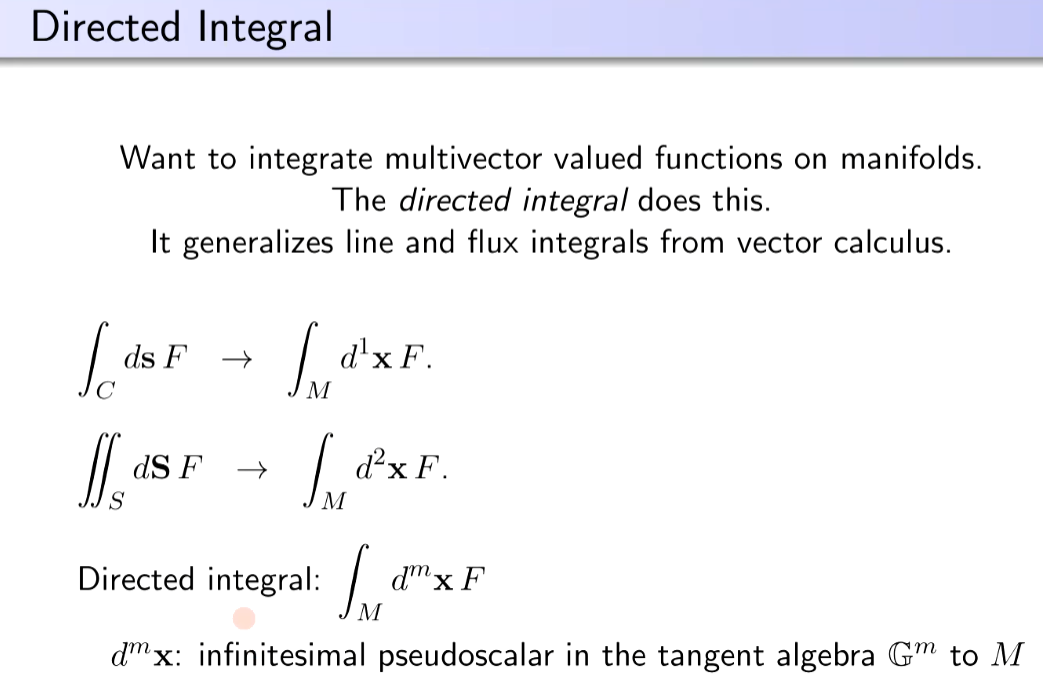
Directed Integral
微積分除了微分還要積分。
Fundamental Theorem of GA Calculus
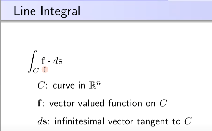
Vector Calculus
GA 可以合爲一體!
$\nabla A = \nabla \cdot A + \nabla \wedge A $
$\int\int\int \nabla A \,dx dy dz = \int\int A\cdot ds + ?$
What’s the physical insight of GA calculus?