Reference
Stokes’ Theorem on Manifolds (youtube.com) : 非常好的 lecture to combine vector calculus!
Vector calculus
Matrix calculus: The Matrix Calculus You Need for Deep Learning - Part 1 (youtube.com) for deep learning
Tensor calculus: refer to youtube, Princeton professor (Burton?)
Differential calculus: refer to visual differential calculus
Geometric algebra, GA (calculus?): refer to youtube
Takeaways

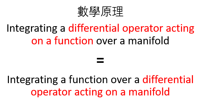
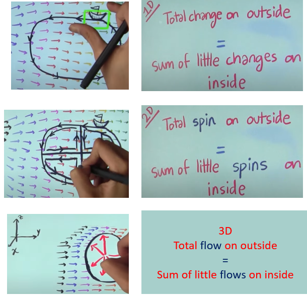
- 微積分可以歸納成一個基本原理:“total change on outside = sum of little changes on inside”
-
不要小看這句話,左邊代表 global property (全域特性,例如拓撲特徵,對稱性,奇點)。右邊代表 local property (局部特性/分析,例如斜率,梯度,旋度,散度,甚至曲率)
-
如果是有源 (source or sink),有兩種處理方式:(1) “total change on outside = sum of little changes on inside + source/sink generation rate”; (2) 加上新的邊界把 source/sink 變成 outside. Cauchy 就是這方面的高手 (複分析)。
-
-
另一個很有深意微積分定理看法是函數的微分,變成幾何的微分。
-
廣義 Stokes Theorem : \(\int_{\partial M} F = \int_M dF \quad \text{or} \quad \int_{\partial M} F = \int_M \partial F\)
-
等式右邊 “sum of little change on inside” 就是 integrating a differential function on a manifold = $\int_M dF $.
- 等式左邊 “total change on outside” 則是 integrating function along the manifold boundary = $\int_{\partial M} F $
- 右邊是 local property, 每一個點的特性都 count。左邊是 global property, 因爲只要管函數在 manifold edges (global) 的特性.
-
Q&A
- Discrete scan method for recursive equation 是微積分概念嗎?
Introduction
積分很自然,就是算面積。從幾千年前的中國和希臘就有這樣的實際需求和問題。
微分是什麽?爲什麽微分和積分牽扯在一起?
一般說微分是斜率,甚至衍生到斜率為 0 就是求極大值和極小值。
問題是斜率和積分有什麽關係。
有!就是微積分定理把算面積的積分和算斜率或是極大/小值的微分結合。這是否很不直觀?
Vector Calculus
從 vector calculus 反而可以看出微積分的基本大法!
- 微分:就是進入無限小體積的流 - 出無限小體積的流的差,也就是無限小體積的微分的流入扣掉流出!
- 積分:既然有流出扣掉流入,根據物質不滅定律,一定有物質在這無限小體積纍積,就是一小部分的積分。
- 最後算總積分就是把所有無限小體積的物質都加起來。
-
微積分定理就是内部互相抵消,只剩下頭尾的兩項。這就是基本大法。
- Divergence 微積分對應的就是體積分變成面積分
- Curl 微積分對應面積分變成綫積分
- Gradient 微積分對應綫積分變成兩點的差值 (這就是大學的微積分定理)!
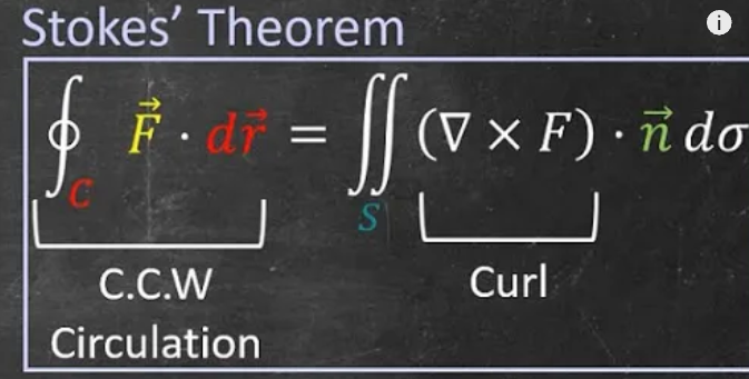
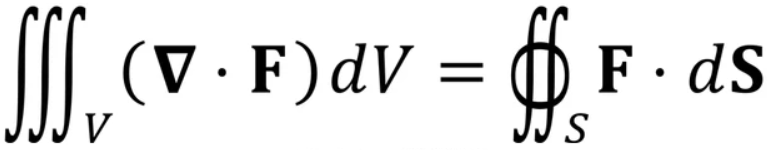
傳統的 Vector calculus 三大定理 (in 3D space):
Gradient Theorem : $\int_a^b \nabla \varphi \cdot d\vec{l} = \varphi(b) - \varphi(a)$
Stokes Theorem : $\iint_S \nabla \times \vec{A} \cdot d\vec{s} = \oint_c \vec{A}\cdot d\vec{l}$
Divergence Theorem : $\iiint_V \nabla \cdot \vec{F} \,dv = \iint_S \vec{F}\cdot d\vec{s}$
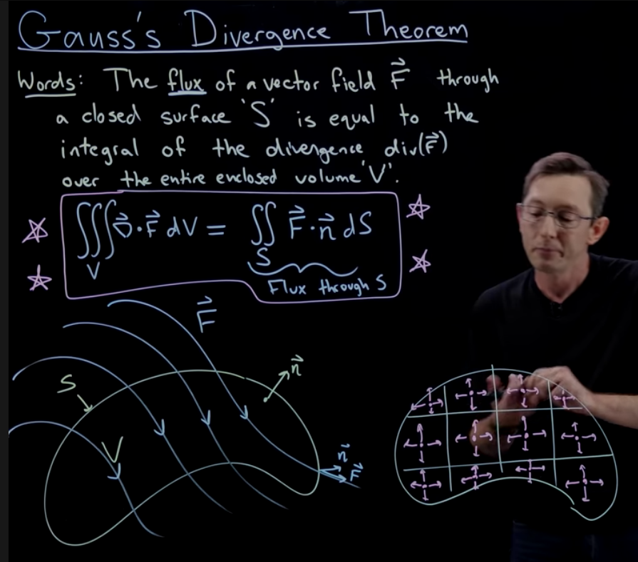
Vector field 的 divergence: 進無限小體積的 - 出體積
我們從最簡單的開始
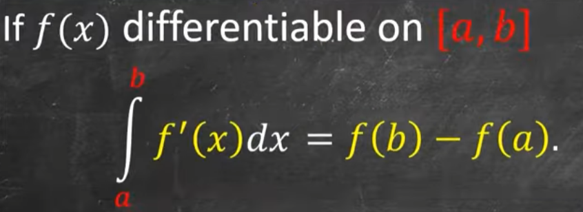
(純量/實分析) 微積分基本定理
- 左邊是 1D little change ($f’(x)$,導數) inside 1D line,右邊是 0D (點) 邊界
(向量場/複分析) 微積分基本定理 (梯度)
-
就是梯度定理。也是 Cauchy 複分析的解析函數微積分定理。
-
左邊是 2D little change ($\nabla f$,梯度) inside 1D line,右邊是 0D (點) 邊界
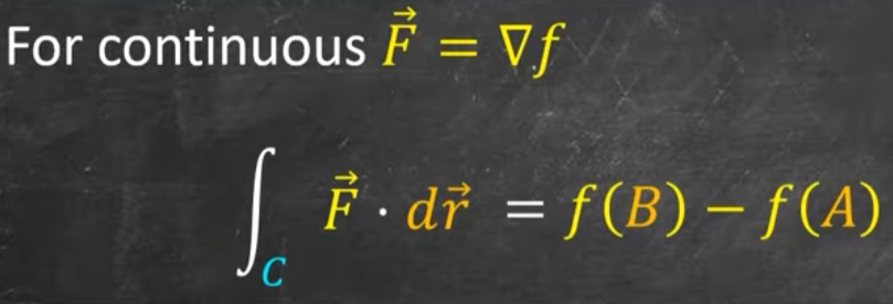
- 如果 y 方向是 uniform/constant field,同時綫積分沿著 y = constant 的方向,梯度定理就化簡成實數的微積分基本定理。物理解釋是内部流量的微分變化,累積成外部邊界的變化。
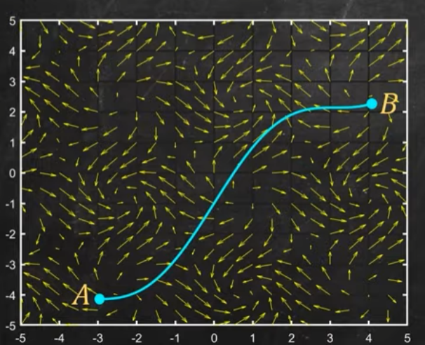
(向量場) 微積分基本定理 (旋度)
- Stokes 定理。右邊是 2D little change ($\nabla\times f$ ,旋度) inside 2D surface,左邊是 1D (環) 邊界

(向量場) 微積分基本定理 (散度)
-
Divergence 定理。左邊是 3D little change ($\nabla\cdot f$ ,旋度) inside 3D volume,右邊是 2D (球) 邊界
另一個解釋:
Curve Space 微積分基本定理 (TBD)
Gauss Theorem on curved space \(\int A^\mu \frac{1}{6} \epsilon^{\mu \nu \rho \sigma} d S_{\nu \rho \sigma}=\int \partial_\mu A^\mu d \Omega\)
Stoke Theorem on curved space \(\frac{1}{2} \int A^{\mu \nu} \frac{1}{2} \epsilon_{\mu \nu \rho \sigma} d F^{\rho \sigma}=\int \frac{\partial A^{\mu \nu}}{\partial x^\nu} \frac{1}{6} \epsilon_{\mu \nu \rho \sigma} d S^{\mu \rho \sigma}\)
Where $d \Omega=d x^0 d x^1 d x^2 d x^3$ is the invariant spacetime volume and $d S_{\mu \rho \sigma}$ ( and $d S^{\mu \rho \sigma}$ ), $d F^{\rho \sigma}$ are 3 -surface and 2 -surface elements, respectively.
這個 “total change on outside = sum of little changes on inside” 的想法,還可以應用在任何可以内部互相抵消的應用。Gauss-Bonnet Theorem 就是一個例子。整理重點
- 這個特性是 additive: 例如梯度,旋度,散度
- 這個特性是可以互相抵消!
彎曲空間的基本定理 (曲率 - Gauss-Bonnet Theorem)
我們在另一個文章再展開。 \(\int_M K d A+\int_{\partial M} k_g d s=2 \pi \chi(M)\)
K 是高斯面曲率,$k_g$ 是 geodesic curvature。基本上 $K = \kappa_1 \kappa_2$。$K$ 和 $k_g$ 并不是直接微分的關係,但是
“total change on outside = sum of little changes on inside”。之後好好推導一下!
\[\begin{gathered} \mathrm{d} \hat{\mathrm{s}}^2=\mathrm{A}^2 \mathrm{~d} \mathrm{u}^2+\mathrm{B}^2 \mathrm{~d} v^2 . \\ K=-\frac{1}{\mathrm{AB}}\left(\partial_v\left[\frac{\partial_v \mathrm{~A}}{\mathrm{~B}}\right]+\partial_{\mathrm{u}}\left[\frac{\partial_{\mathrm{u}} \mathrm{B}}{\mathrm{A}}\right]\right) . \\ \mathrm{d} \hat{\mathrm{s}}^2=\Lambda^2\left[\mathrm{du}+\mathrm{d} v^2\right] . \\ \mathcal{K}=-\frac{\nabla^2 \ln \Lambda}{\Lambda^2} . \end{gathered}\]