Reference
(1) The Fisher Information - YouTube [@mutualinformationFisherInformation2021] - good reference
MLE (Maximum likelihood estimation) 就是 (n-sample) likelihood function 微分為 0 => 可以 estimate parameter, easy!
問題是這個 estimated parameter 的 quality 到底好不好?需要有一個度量: (1) 是否會 converge to true value (consistency), (2) 假設會 converge, 要多少 samples 才能 converge to given accuracy. 這就是 Fisher 和 Fisher information, Cramer-Rao bound 要解決的問題。
Score and Fisher Information 非常多 confusing 點:
-
Likelihood function 到底是 1-point probability function, 或是 N repeated joint probability function?
Ans: In general n-samples, but often set n=1 for theoretical derivation
-
Score function 的幾何或是物理意義是什麽? D-log-likelihood function.
Ans: Likihood function 的微分。likelihood 斜率為 0 的點,對應 maximum likelihood 點,是 score function 的 0 點。
Ans: 重點是 score function 對 x 的平均為 0, 方差卻是一個穩定的數稱為 Fisher information. 愈大代表估計愈好。
-
爲什麽 Fisher information = var = -1 * 2nd order derivative? Fisher Information 的意義是什麼?
Ans: Score function 在 0 值 distribution 的 variance
Ans: 曲率,大代表好的鑑別度。
-
到底 variance 大比較好 estimate? (yes), 似乎 counter intuitive!! Variance 小比較好 estimate?
Ans: Depends on which variance!!!
-
What’s Fisher Information related to (Mutual) Entropy?
-
How Fisher Information related to Manifold Geometry Learning?
-
Bayesian 也有 Fisher information 嗎?
Ans: Yes
Introduction
Parameter Estimation 在統計學應用非常廣,通訊、控制、機器學習中的 regression and classification, etc. 都會應用到。最常使用的 paramter estimation 是 Maximum Likelihood estimation (ML or MLE).
MLE 的觀念和求解非常簡單:從 probability distribution with parameter $\theta$ 出發。根據 samples 定義 likelihood or log likelihood function. $\theta_{ML}$ 就是解 likelihood or log likelihood function 的一階導數為 0.
問題是這個 parameter estimation 的 quality 到底好不好?需要有一個度量,這就是 Fisher 在 19xx 的 work, 包含 score function 和 Fisher information.
Distribution and Sample
統計 (Statistics) 和機率最大的差異:機率強調 distribution, 比較偏向理論。統計把 samples and distribution 並重,更強調實務。Sample 基本對應 likelihood function.
Example: 從最簡單的 Bernoulli distribution (experiment) 開始: 假設銅板出現 head (success) 的機率是 $\theta_o$, 如何從 n 次 samples (or observations or evidences) 估計出 $\theta_o$?
重複丟銅板,丟出 A 次 head and B 次 tail (n = A+B). $x_1, x_2, \ldots, x_n$ 都是 observed outcome. 直覺的estimation 就是 $\hat{\theta} = \frac{A}{A+B} = \frac{A}{n} \sim\text{ true prior } \theta_o$
如何 justify 這個結果? 如果 n 夠大,從大數法則就可看出。但如果 n 不大,或是 estimated parameter 並非 mean 而是其他參數 (e.g. variance, or probability in logistic regression), 就需要更有系統的理論支撐。這就是 Fisher 在二十世紀的工作,從 likelihood function 到 score function 和 Fisher information.
Likelihood Function
以下是 likelihood function 的定義:
- $Z \sim p\left(z ; \theta_0\right) . \theta_o \in \Re^K . p(z ; \theta)$ is a member of a parametric class ‘indexed’ by $\theta$.
- $\tilde{Z}=\left(Z_1, Z_2, \ldots, Z_n\right)^{\prime}$ is an iid sample $\sim p\left(z ; \theta_0\right)$. The likelihood function for $Z$ is \(L(\theta ; z): \Re^K \rightarrow \Re: p(z ; \theta) \label{Like1}\) In the density function $\theta$ is taken as given and $z$ varies. In the likelihood function these roles are reversed Note that due to the iid assumption: \(L(\theta ; \tilde{z})=p(\tilde{z} ; \theta)=\Pi_{i=1}^n p\left(z_i ; \theta\right)=\Pi_{i=1}^n L\left(\theta ; z_i\right) \label{LikeN}\) 通常我們會再定義 log-likelihood function, $l(\theta; z)$, 簡化乘法變成加法以及讓微分更容易。 \(l(\theta ; \tilde{z})=\log p(\tilde{z} ; \theta)=\log \Pi_{i=1}^n p\left(z_i ; \theta\right)=\Sigma_{i=1}^n \log p\left(z_i ; \theta\right)=\Sigma_{i=1}^n l\left(\theta ; z_i\right) \label{LogLikeN}\) Q: Likelihood function 是 1-sample probability distribution, 或是 N iid-sample joint probability function?
Ans: Likelihood function 就是 probability distribution function of (parameter) $\theta$ with n samples. 其實和 (joint) probability distribution function 是一體兩面:差異是 samples 是已知,parameter 是未知需要從 sample 估計。如果是 n iid experiment, 則對應 joint probability distribution. Likelihood function (and Score function, Fisher Information) 一般是指 n iid-sample joint pdf. 因爲一個 sample 基本很難做 parameter estimation! 不過把 n = 1 就化簡成 1-sample probability distribution, 看起來比較習慣簡單。
$\eqref{LikeN}$ 把 $n=1$ 就化簡成 $\eqref{Like1}$. 不過在理論推導時一般常常默認 n = 1,因爲 n 是 sample number, depends on the real scenario. 默認 n = 1 可以簡化推導。不過實務上要 n samples 才能做 parameter estimation.
Example: $Z \sim N\left(\mu, \sigma^2\right)$ Here $\theta=\left(\mu, \sigma^2\right)$, and $K=2$. Note:
-
$p(z ; \theta): \Re \rightarrow \Re: \frac{1}{\sqrt{2 \pi} \sigma} \exp \left[-\frac{(z-\mu)^2}{2 \sigma^2}\right]$
-
$L(\theta ; z): \Re^2 \rightarrow \Re: \frac{1}{\sqrt{2 \pi} \sigma} \exp \left[-\frac{(z-\mu)^2}{2 \sigma^2}\right]$
Intuitively, $L\left(\theta ; z_0\right)$ quantifies how compatible is any choice of $\theta$ with the occurrence of $z_0$.
Maximum likelihood estimation 就是一階導數 of likelihood function 為 0 的解:$D L(\hat{\theta}; \tilde{z}) = L’(\hat{\theta}; \tilde{z}) = 0 \to \hat{\theta}$. 因爲 log 是 monotonic function, Maximum likelihood estimation 等價與 maximum log-likelihood estimation. 也就是$ D l(\hat{\theta}; \tilde{z}) = l’(\hat{\theta}; \tilde{z}) = 0 \to \hat{\theta}.$
因爲 log-likelihood function 一階微分非常重要,特別定義 Score function = 一階微分 of log-likelihood function **, $s(\theta; \tilde{z}) = D \log L(\theta; \tilde{z}) = D l(\theta;\tilde{z}) = l’(\theta;\tilde{z})$. **後面很多重要的統計特性都和 Score function 相關!
Bernoulli Distribution Log/Likelihood and Score Function (n-samples)
Likelihood function:$L(\theta) = \theta^{A} (1-\theta)^{B}$ where $A+B = n$
Likelihood 一階微分: $L’(\theta) = A \theta^{A-1}(1-\theta)^{B} - B\theta^A (1-\theta)^{B-1}$
找 maximum likelihood: $L’(\hat{\theta}) = 0 \to A \hat{\theta}^{-1} - B (1-\hat{\theta})^{-1} = 0 \to \hat{\theta} = \frac{A}{A+B} = \frac{A}{n}$
Log-likelihood function: $l(\theta) = \log L(\theta) = A \log \theta + B \log (1-\theta)$
Score function = Log-likelihood function 一階微分: $s(\theta) = l’(\theta) = \frac{A}{\theta} - \frac{B}{1-\theta}$
找 maximum log-likelihood: $l’(\hat{\theta}) = s(\hat{\theta}) = 0 \to \hat{\theta} = \frac{A}{n}$ 結果和 maximum likelihood 一樣, as expected.
Gaussian Distribution Log/Likelihood and Score Function (n-samples)
接著看 continuous 的例子: the likelihood function \(L\left(\mu, \sigma^2 ; x_1, \ldots, x_n\right)= \Pi_{i=1}^n p\left(z_i ; \theta\right)= \left(2 \pi \sigma^2\right)^{-n / 2} \exp \left(-\frac{1}{2 \sigma^2} \sum_{j=1}^n\left(x_j-\mu\right)^2\right)\) 明顯 likelihood function 很難處理。因此一般用 log-likelihood function \(l\left(\mu, \sigma^2 ; x_1, \ldots, x_n\right)= \Sigma_{i=1}^n \log p\left(z_i ; \theta\right)= -\frac{n}{2} \ln (2 \pi)-\frac{n}{2} \ln \left(\sigma^2\right)-\frac{1}{2 \sigma^2} \sum_{j=1}^n\left(x_j-\mu\right)^2\)
對 log-likelihood function 做一階 (偏) 微分並設爲 0, 可以解出 mean and variance 的 maximum likelihood estimates:
\[\begin{align} &\widehat{\mu}_n=\frac{1}{n} \sum_{j=1}^n x_j \label{Mean}\\ &\hat{\sigma}_n^2=\frac{1}{n} \sum_{j=1}^n\left(x_j-\widehat{\mu}\right)^2 \label{Var} \end{align}\]Maximum Likelihood Estimation
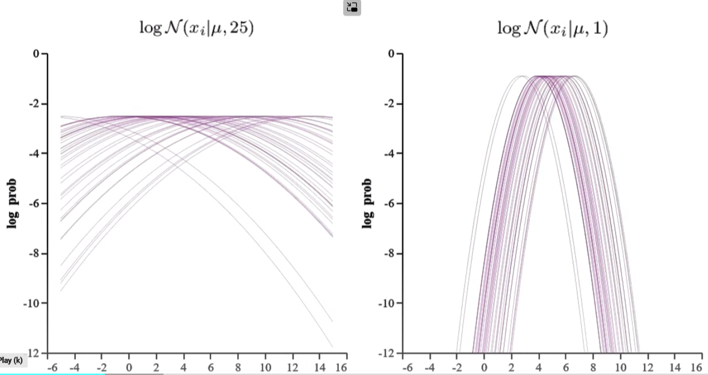
先簡化問題:如果 normal distribution 的 variance 已知,我們只有一個 parameter mean, $\mu$, 需要估計。假設有兩個 normal distributions 有不同 variance (e.g. $\sigma = 1$ or $\sigma = 25$) 但是相同 mean (e.g. $\mu_1 = \mu_2$) to be estimated. 也就是有兩組 n samples 來自兩個 normal distributions 做爲 mean estimation.
我們知道 maximum likelihood estimation (MLE) $\hat{\mu}$ in $\eqref{Mean}$ 是”符合直覺“的估計值。但這兩組 n-samples 的估計, 那一組的 MLE 的準確度比較高?或者如何判斷 MLE 的”quality”? 以上就是 Fisher 在提出 MLE 同時想解決的問題。
Fisher 的想法:
- 爲什麽 MLE 是”符合直覺“ 的 estimation? $\Rightarrow$ Consistency, MLE converges to true value when $n \to \infty$
- 如何度量 MLE quality? $\Rightarrow$ Accuracy with bound
- 換一個角度,假設 MLE 會 converge 到 true value when $n \to \infty$. $\Rightarrow$ Accuracy 的 metric 可以改成 efficiency, 就是用比較少的 sample 達到要求的 accuracy.
Visualize n-Sample Log-Likelihood 和 Score functions (精華)
簡單的想法就是做 n 次實驗看 distribution, 如何進行?
一個 sample (n=1) 的 likelihood function 很難有什麽直覺。反之 n-維空間的 likelihood function 無法想像。一個非常有用的方法: accumulate “n 個 1-sample 的 log-likelihood function!” 爲什麽要用 log-likelihood? 除了 dynamic range 比較小容易 visualize; 同時計算容易,從 1-sample to n-samples (的 log-likelihood function, score function, and Fisher information) 只需要 summation 或是乘 n.
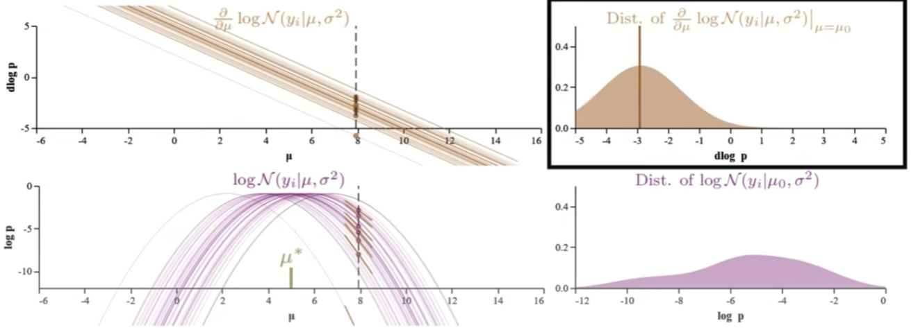
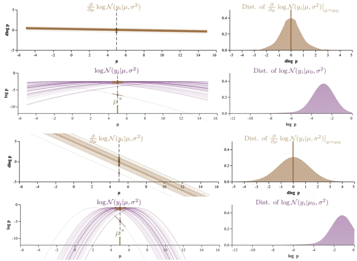
我們以下兩個 log-likelihood function of normal distribution 爲例。左圖的 $\sigma^2 = 25$; 右圖的 $\sigma^2=1$; 目的是估計兩個 functions 的 $\hat{\mu}$ (true mean 都是 5). 左右圖中的每一條 trace 都對應 1-sample 的 log-likelihood function. 右圖肉眼可以猜出 $\hat{\mu}=5$. 左圖則很難猜出 $\hat{\mu}=5$,可能要更多的 traces.
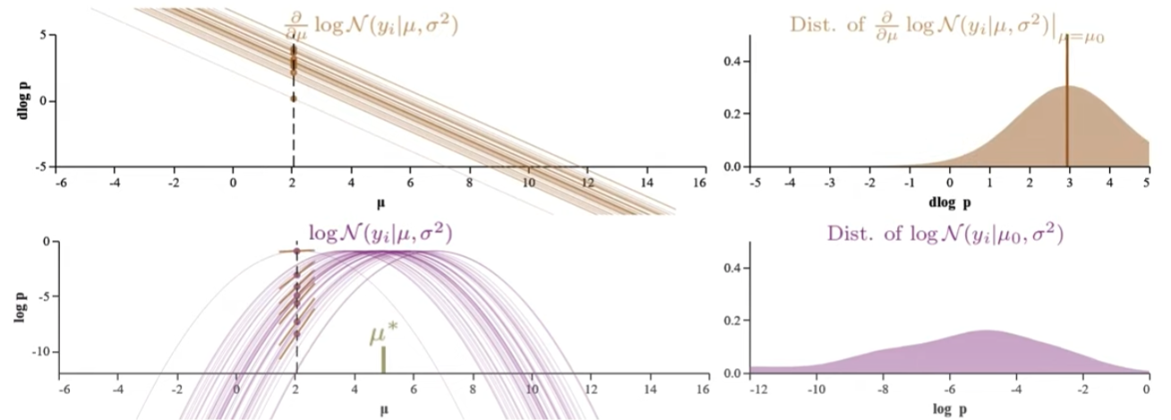
我們對於右圖 $\sigma^2=1$ 深入研究:對於每一個 (estimated) fixed $\mu$ 垂直切綫看 n-samples/traces log p 的分佈,如左下圖。並且把這個分佈視爲一個 probability distribution 畫在右下圖 (每一個 distribution 對應一個特定的 $\mu$)! 有了 distribution, 之後就可以計算 mean, variance, etc.
爲什麽是固定 $\mu$ 看 distribution? 因爲在 MLE $\mu$ 是 fixed parameter 而不是 distribution (Bayesian)! 因此統計的特性 (expectation value, like mean, variance, etc.) 還是對 $p(x)$ given $\mu$, or $p(x; \mu)$!!
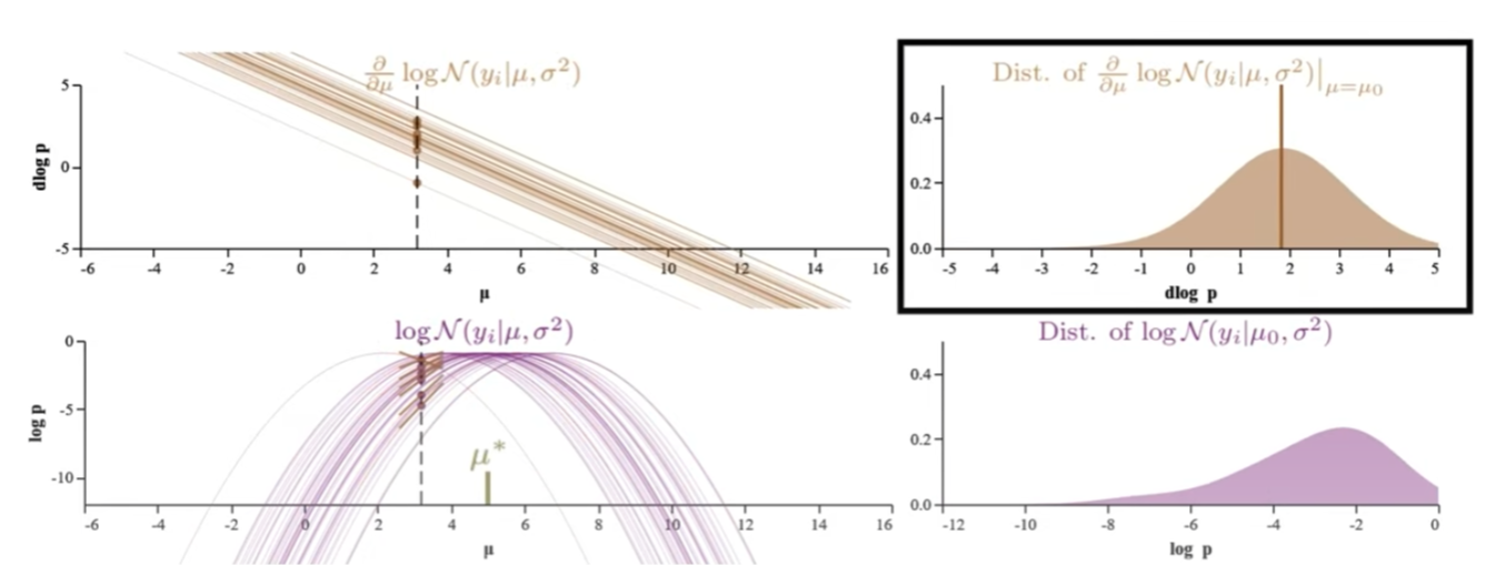
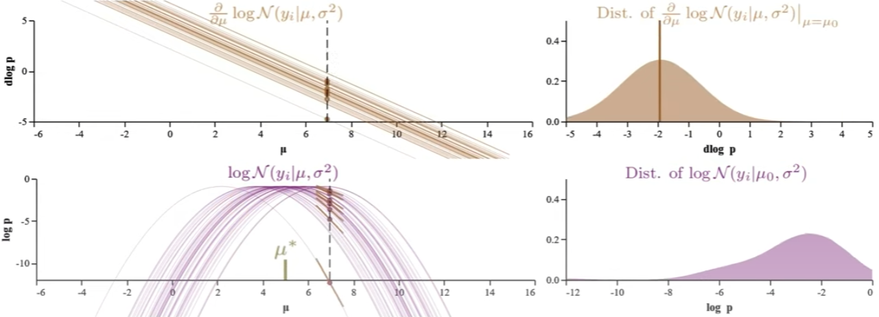
| 下面共有五組圖都對應 $N(x | \mu,1)$:每組包含其 log-likelihood function (左下) 和 score function (log-likelihood一階微分, 左上) 以及右邊對應的 n-sample distribution at fixed $\mu$. 從上到下,五組 $\mu$ = {2, 3, 5, 7, 8}. 注意 $\hat{\mu} = 5$ 1. |
-
Normal distribution 的 log-likelihood function (左下) 是抛物綫,score function (左上) 是直綫 with negative slope.
-
Log-likelihood function 的 log-p distribution (右下):可以看出 (或是想象出) $\mu$ 約接近 $\hat{\mu}$ 時,log-p distribution 約 compact, 並且在 $\mu = \hat{\mu}$ 有最小 log-p variance. 不過 log-p distribution 隨 $\mu$ 變化很大,似乎比較難 extract stable information. 以下的 score function 更有用!
-
Score function 的 D-log-p (log-likelihood 的斜率) distribution (右上):記住 score function 為 0 的解就是 $\hat{\mu}$. $\hat{\mu}$ 對應 log-likelihood 的極大值 of 斜率為 0. 所以 $\mu$ 約接近 $\hat{\mu}$, D-log-p (log-likelihood 的斜率) 的 distribution 的 mean 約接近 0. But why the D-log-p distribution mean 剛好為 0? 需要進一步證明 $\hat{\mu}$ 對這個 D-log-p distribution 的平均值為 0.
- 更重要的是 Score function 的 D-log-p distribution 的形狀 (therefore D-log-p variance) 五組都一樣。 當然完全一樣是 normal distribution 的特例,因爲 normal distribution score function 剛好是直綫。對於其他的 probability distribution,variance 雖然會變化,但在 $\hat{\mu}$ 附近也是一個比較穩定值。Score function 的 variance 稱爲 Fisher Information 永遠大於 0, 非常重要!

Fisher Information Deep Dive
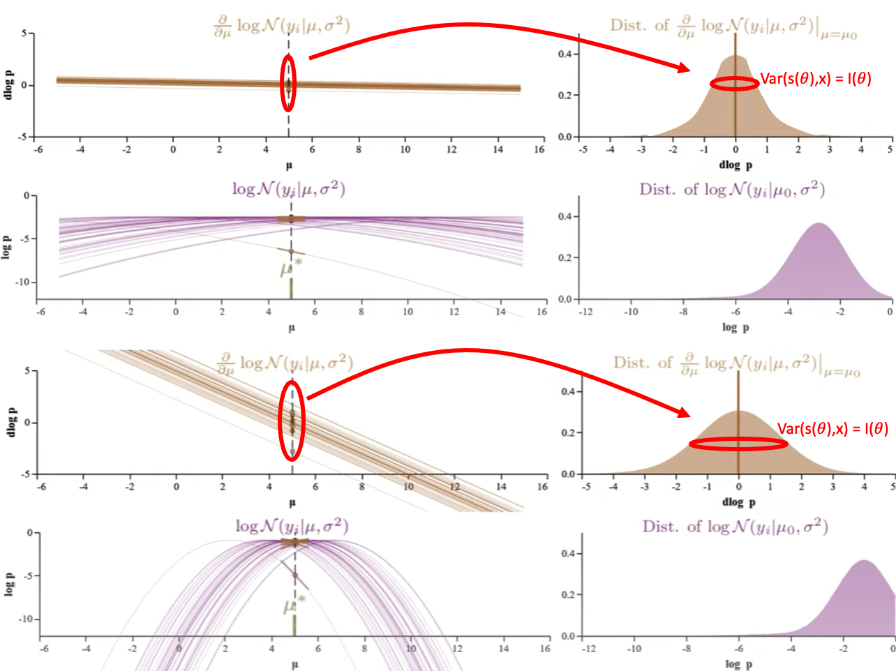
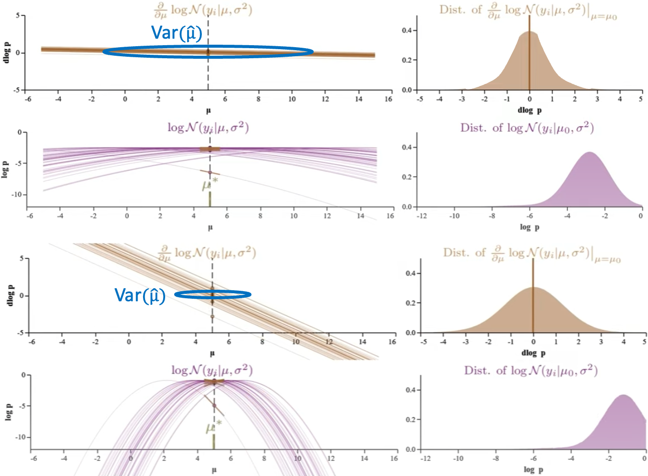
| 如何 visualize D-log-P variance (i.e. Fisher Information) 影響 parameter estimation? 我們再仔細比較下圖 $N(x | \mu,25)$ 和下下圖 $N(x | \mu,1)$ 的例子。兩個 normal distributions 的 true mean 都是 5. 很明顯 normal distribution of $\sigma^2=25$ 比較難準確估計 $\mu$! 比較下圖右和下下圖右的 Score function D-log-P 分佈 variance (i.e. Fisher Information) at a fixed $\mu$, $\sigma^2=25$ 的 卻比 $\sigma^2=1$ 的 D-log-P variance 小!! |
Fisher Information (or D-log-P variance) 和 maximum likelihood estimated parameter $\hat{\mu}$ 的準確度正相關。 Fisher Information 越大,i.e. D-log-P 的 variance 越大,代表 MLE 估計約準確! 愈大的 Fisher Information 估計愈準確,愈有鑒別力。
Why Fisher information = (-1) * Log-likelihood 2nd derivative? Fisher Information 意義是什麼?
另一個有趣的點: Log-likelihood 二階微分, i.e. D-D-log-p 在 $\hat{\mu}$ 的二階導數 (正比曲率) 剛好等於負的 Fisher Information, why?? \(I(\theta) = Var( D \log p(x; \hat{\mu})) = E(D \log p(x; \hat{\mu})^2) = - E(D^2 \log p(x; \hat{\mu}))\)
- 上圖可以看出 log-likelihood 的二階導數開口向下是負數。但是 Fisher Information (Variance) 永遠是正的,所以會差一個負號。
- Log-likelihood function 在 $\hat{\mu}$ 的曲率 (2nd order derivative) 數值愈大,約有鑒別力。這和 Fisher Information 有異曲同工之妙!
這是 Fisher Information 的 physical insight,Fisher Information 基本等價 log-likelihood function 在 $\hat{\mu}$ 的曲率 with a negative sign. 所以 Fisher Information 愈大,愈有鑑別度。
| 下一個重要發展是 Cramer-Rao bound, i.e.可以證明 (Wrong!) $ | \theta - \hat{\theta} | \le 1/I(\theta)$. 正確的 Cramer-Rao bound: |
-
Fisher information 愈大,maximum likelihood estimated parameter variance 愈小,就愈準確。
-
Cramer-Rao bound 是 lower bound:也就是 MLE parameter 不可能做的比 Fisher Information 的倒數更好。Normal distribution 的 mean estimation 等號成立。
三種 Variance Demystify
進一步 deep dive Fisher Information 和 MLE 的 accuracy and efficiency 會牽扯到不同的 variance, 所以我們先對三種不同 variance(s) demystify:
-
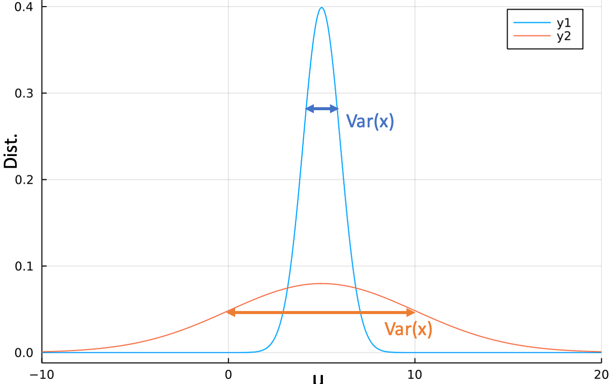
第一個 variance 指原始 probability distribution, $p(z ; \theta)$, 或是 likelihood function, $L(\theta ; z)$, 的 variance. 如上圖 normal distribution, $N\left(\mu, \sigma^2\right)$, 的 $\sigma^2$. 下面兩圖比較 $\sigma^2 = 25$ (top) 和 $\sigma^2 = 1$ (bottom) 估計 $\mu$ (=5). 如果是 estimate mean ($\mu$) of the likelihood function. 顯然 variance 愈大愈難估計的準確,或者 variance 愈大要更多的 sample 才能得到同樣的準確度。
-
第二個 variance 是指 fixed parameter 從垂直割綫看 log-p (log-likelihood) 或是 D-log-p (score function) 分佈 variance (右圖紅圈)。此時 variance 作用和第一類 variance 相反!垂直割綫的分佈方差愈大,代表鑒別能力愈好,愈容易估計準確! Fisher Information 即是 D-log-p 對應 $\hat{\mu}$ 的垂直割綫方差!以下圖的兩個例子 $\sigma^2 = 25$ (top) 比 $\sigma^2 = 1$ (bottom) 更難估計 $\mu$. Appendix A 推導 normal distribution 的 score function 的垂直割綫 variance, 剛好是第一類 variance 的倒數。
- $Var[s(\theta ; x)] = I(\theta) = \frac{1}{\sigma^2}$ (1-sample) Fisher Information 剛好和 normal distribution 的 variance (上圖) 相反!
因此會有一個乍看很奇怪的結論: Fisher information 愈大 (代表上圖的 normal distribution variance 愈小),愈容易估計的準確。
- 第三個 variance 是 estimated parameter 的 variance. 如下圖 score function 的水平割線 @ $\hat{\mu}$。 一個直觀看法就是 fixed log-p 從水平割綫看 $\mu$ 的分佈方差,愈大愈難估計準確。比較 $\sigma^2 = 25$ (top) 和 $\sigma^2 = 1$ (bottom) 的 score function, 顯然 variance 愈大愈難估計的準確。這和第一個 (probability distribution) variance 的結論一致,但和第二個 (D-log-p, score function distribution) variance 剛好相反。第三個 variance 有一個 metric, Cramer-Rao bound, 規範了第三個 variance!
- $Var(\hat{\theta}) \ge \frac{1}{I(\theta)}$
注意以上都是 1-sample Fisher Information. 實務上 n-sample 只要把 Fisher information 乘 n 即可。
Fisher Information vs. Shannon Information
-
理論上用 log-likelihood function 斜率為 0, 也就是 Score function 為 0 解出 $\hat{\mu}$. 實務上用 samples average 估計 $\hat{\mu}$.
-
- $l’(\mu; x) = \frac{d \log p(x; \mu)}{d \mu} = s(\mu; x)= 0 \to \hat{\mu}$ 是 maxmimum likelihood estimation
- Score function 在 $\hat{\mu}$ 的 mean 為 0: $E(s(x; \hat{\mu})) = 0$: 雖然直觀,need to prove it.
- $E(s(x; \hat{\mu})) = \int s(x; \hat{\mu})$
- Score function 的 variance 很穩定不隨 $\mu$ 有太多改變,並且 $Var(score(x; \hat{\mu}))$ 可以代表 estimation 的準確度,稱爲 Fisher information! 實務上應該可以用 samples variance 估計 $\hat{\mu}$ 的 efficiency? YES!!!! 這就是 Rao-Cramer bound, $Var(\hat{\mu}) \ge 1$
- log-likelihood variance 隨 $\mu$ 變化大,在 $\hat{\mu}$ 的 variance 最小,不過這個似乎有點難用?
Appendix
Appendix A: Normal Distribution Score and Fisher Information Example
\[\begin{align} &p(x; \theta)=\mathcal{N}(x; \theta, \sigma^2)=\frac{1}{\sqrt{2 \pi} \sigma} \exp\left[-\frac{(x-\theta)^2}{2 \sigma^2}\right] \nonumber\\ &l(\theta; x)= \log p(x; \theta)= - \log{\sqrt{2 \pi} \sigma} - \frac{(x-\theta)^2}{2 \sigma^2} \quad\text{(1-sample log-likelihood)}\nonumber\\ &s(\theta ; x)=\frac{d l(\theta; x)}{d \theta} =\frac{-(\theta-x)}{\sigma^2} \quad\text{(1-sample score \& Neg. slope inversely prop. to variance)}\label{Score}\\ &D^2\,l(\theta; x)= D\,s(\theta; x) = - \frac{1}{\sigma^2} \,\text{(1-sample 2nd derivative of log-likelihood = -Fisher Inform.)}\label{Curv}\\ \end{align}\]以上只是 1-sample for $x$, 如果有 n-sample $s(\theta; x_1, \ldots, x_n)$, $x_1, \ldots, x_n$ 的 sample distribution 會是什麽? 如果 $n\to\infty$, 這個 distribution 趨近 true distribution (e.g. $\mathcal{N}(x;5,\sigma^2)$ in the example). 當然因爲我們並不知道 true distribution, 因此只能用 MLE $\mathcal{N}(x;\hat{\theta},\sigma^2)$ 近似。
\[\begin{aligned} &E[s(\theta ; x)]= E\left[\frac{-(\theta - x)}{\sigma^2}\right] \\ &= \int \frac{-(\theta - x)}{\sigma^2} \frac{1}{\sqrt{2 \pi} \sigma} \exp\left[-\frac{(x-\hat{\theta})^2}{2 \sigma^2}\right] d x\\ &= \frac{\hat{\theta} - \theta}{\sigma^2}\\ \end{aligned}\] \[\begin{aligned} &Var[s(\theta ; x)]= Var\left[\frac{-(\theta - x)}{\sigma^2}\right] \\ &= Var\left[\frac{x}{\sigma^2}\right] = \frac{ Var[x]}{\sigma^4} = \frac{\sigma^2}{\sigma^4} \\ &= \frac{1}{\sigma^2} \end{aligned}\]Score function 的平均值是負斜率 ($-1/\sigma^2$), 和 x-軸相交在 $\hat{\theta}$.
Score function 平均值在 MLE $\hat{\theta}$ 為 0, $E[s(\theta ; x)]_{\hat{\theta = \theta}} = 0$
Score function 的方差是 ($1/\sigma^2$), a constant at any $\theta$.
Log-likelihood function 的平均和方差就不顯示推導結果,只顯示 Log-likelihood function 的平均
\(\begin{aligned} E[l(\theta ; x)]= -\log\sqrt{2\pi} \sigma - \frac{1}{2}- \frac{1}{2\sigma^2}(\hat{\theta}-\theta)^2 \end{aligned}\) 可以對照五組圖的 Score function 的平均值如下表:
| Score (D-log-p) 平均 | Score (D-log-p) 方差 (i.e. Fisher Inf.) | Log-Likelihood (log-p) 平均 | |
|---|---|---|---|
| 2 | 3 | 1 | -5.9 |
| 3 | 2 | 1 | -3.42 |
| 5 | 0 | 1 | -1.42 |
| 7 | -2 | 1 | -3.42 |
| 8 | -3 | 1 | -5.9 |
Reference
-
公式推導和數值見 Appendix A ↩