Main Reference
- [@santamariaEntropyMutual2015]
Introduction
Shannon 開啟 Information Theory 提供一個定量 measure information (or uncertainty) 的方法,即是 entropy.
Information theory 給了 noisy channel capacity, set the fundmental limitation of (digital) communication theory.
Information theory or entropy 在 machine learning 也是一個重要的 guiding principle, e.g. maximum entropy principle.
(Self)-Entropy
分成 continuous variable or discrete random variable.
Discrete Random Variable
Self-entropy 的定義如下 \(\mathrm{H}(X)=-\sum_{i=1}^{n} \mathrm{P}\left(x_{i}\right) \log \mathrm{P}\left(x_{i}\right)\) 幾個重點:
- 因為 $\sum_{i=1}^{n} \mathrm{P}\left(x_{i}\right) = 1$ and $1\ge \mathrm{P}(x_{i})\ge 0$, 所以 discrete RV 的 entropy $H(X) \ge 0$. (注意,continuous RV 的 entropy 可能會小於 0!)
- Log 可以是 $\log_2 \to H(x)$ 單位是 bits; 或是 $\log_e \to H(x)$ 單位是 nat; 或是 $\log_{10} \to H(x)$ 單位是 dits.
Example 0: Bernoulli distribution ~ B(p)
0 <= H(X, p) <= 1, unit bits

Continuous Random Variable
Self-entropy 的定義如下 \(\mathrm{H}(X)=-\int p\left(x\right) \log p\left(x\right) d x\) 幾個重點:
- 因為 $\int p\left(x\right) d x = 1$. 重點是 $p(x) \ge 0$ , 但 $p(x)$ 可以大於 1. 所以注意,continuous RV 的 entropy 可能會小於 0!
- Log 可以是 $\log_2 \to H(x)$ 單位是 bits; 或是 $\log_e \to H(x)$ 單位是 nat; 或是 $\log_{10} \to H(x)$ 單位是 dits.
Example 1: Entropy of a uniform distribution, X ∼ U(a, b)
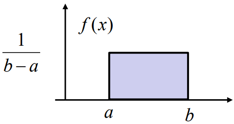
$H(X) = \log (b-a)$
Note that $H(X) < 0$ if $(b-a) < 1$
Example 2: Entropy of a normal distribution, $X \sim N(0, \sigma^2)$
$H(X) = \log (2\pi e \sigma^2)$
Note that $H(X) < 0$ if $2\pi e \sigma^2 < 1$

Maximum Entropy Distribution
For a fixed variance ($Var[X] = E[X^2]-E[X]^2 = \sigma^2$), the normal distribution is the pdf that maximizes entropy.
\(\begin{array}{ll} \underset{f(x)}{\operatorname{maximize}} & -\int f(x) \log f(x) d x \\ \text { subject to } \quad & f(x) \geq 0 \\ & \int f(x) d x=1 \\ & \int x^{2} f(x) d x=\sigma^{2} . \end{array}\) This is a convex optimization problem (entropy is a concave function) whose solution is \(f(x)=\frac{1}{\sqrt{2 \pi} \sigma} e^{-\frac{x^{2}}{2 \sigma^{2}}}\)
Example 1: Communication Channel. Discrete Mutual Information
| I(X; Y) = D (f(x,y) , f(x)f(y)) = H(X) - H(X | Y) |
 \(\begin{aligned}
&I(X ; Y)=h(Y)-h(Y \mid X) \\
&h(Y)=\frac{1}{2} \log \left(2 \pi e\left(\sigma_{x}^{2}+\sigma_{n}^{2}\right)\right) \\
&h(Y \mid X)=h(N)=\frac{1}{2} \log \left(2 \pi e \sigma_{n}^{2}\right) \\
&I(X ; Y)=\frac{1}{2} \log \left(1+\frac{\sigma_{x}^{2}}{\sigma_{n}^{2}}\right)
\end{aligned}\)
This is the channel capacity of a AIWG channel.
\(\begin{aligned}
&I(X ; Y)=h(Y)-h(Y \mid X) \\
&h(Y)=\frac{1}{2} \log \left(2 \pi e\left(\sigma_{x}^{2}+\sigma_{n}^{2}\right)\right) \\
&h(Y \mid X)=h(N)=\frac{1}{2} \log \left(2 \pi e \sigma_{n}^{2}\right) \\
&I(X ; Y)=\frac{1}{2} \log \left(1+\frac{\sigma_{x}^{2}}{\sigma_{n}^{2}}\right)
\end{aligned}\)
This is the channel capacity of a AIWG channel.

VAE Loss Function Using Mutual Information
VAE distribution loss function 對於 input distribution $\tilde{p}(x)$ 積分。 $\tilde{p}(x)$ 大多不是 normal distribution.
\[\begin{align*} \mathcal{L}&=\mathbb{E}_{x \sim \tilde{p}(x)}\left[\mathbb{E}_{z \sim q_{\phi}(z | x)}[-\log p_{\theta}(x | z)]+D_{K L}(q_{\phi}(z | x) \| \,p(z))\right] \\ &=\mathbb{E}_{x \sim \tilde{p}(x)} \mathbb{E}_{z \sim q_{\phi}(z | x)}[-\log p_{\theta}(x | z)]+ \mathbb{E}_{x \sim \tilde{p}(x)} D_{K L}(q_{\phi}(z | x) \| \,p(z)) \\ &= - \iint \tilde{p}(x) q_{\phi}(z | x) [\log p_{\theta}(x | z)] dz dx + \mathbb{E}_{x \sim \tilde{p}(x)} D_{K L}(q_{\phi}(z | x) \| \,p(z)) \\ &= - \iint q_{\phi}(z, x) \log \frac{ p_{\theta}(x, z)}{p(x) p(z)} dz dx + \mathbb{E}_{x \sim \tilde{p}(x)} D_{K L}(q_{\phi}(z | x) \| \,p(z)) \\ \end{align*}\]對 $x$ distribution 積分的完整 loss function, 第一項就不只是 reconstruction loss, 而有更深刻的物理意義。
記得 VAE 的目標是讓 $q_\phi(z\mid x)$ 可以 approximate posterior $p_\theta(z\mid x)$, and $p(x)$ 可以 approximate $\tilde{p}(x)$, i.e. $\tilde{p}(x) q_{\phi}(z\mid x) \sim p_\theta(z\mid x) p(x) \to q_{\phi}(z, x) \sim p_\theta(z, x)$.
此時再來 review VAE loss function, 上式第一項可以近似為 $(x, z)$ or $(x’, z)$ 的 mutual information! 第二項是 (average) regularization term, always positive (>0), 避免 approximate posterior 變成 deterministic.
Optimization target: maximize mutual information and minimize regularization loss, 這是 trade-off.
\[\begin{align*} \mathcal{L}& \sim - I(z, x) + \mathbb{E}_{x \sim \tilde{p}(x)} D_{K L}(q_{\phi}(z | x) \| \,p(z)) \\ \end{align*}\]Q: 實務上 $z$ 只會有部分的 $x$ information, i.e. $I(x, z) < H(x) \text{ or } H(z)$. $z$ 產生的 $x’$ 也只有部分部分的 $x$ information. $x’$ 真的有可能復刻 $x$ 嗎?
A: 復刻的目標一般是 $x$ and $x’$ distribution 儘量接近,也就是 KL divergence 越小越好。這和 mutual information 是兩件事。例如兩個 independent $N(0, 1)$ normal distributions 的 KL divergence 為 0,但是 mutual information, $I$, 為 0. Maximum mutual information 是 1-1 對應,這不是 VAE 的目的。 VAE 一般是要求 marginal likelihood distribution 或是 posterior distribution 能夠被儘可能近似,而不是 1-1 對應。例如 $x$ 是一張狗的照片,產生 $\mu$ and $\log \sigma$ for $z$, 但是 random sample $z$ 產生的 $x’$ 並不會是狗的照片。
這帶出 machine learning 兩個常見的對抗機制:
- GAN: 完全分離的 discriminator and generator 的對抗。
- VAE: encoder/decoder type,注意不是 encoder 和 decoder 的對抗,而是 probabilistic 和 deterministic 的對抗 => maximize mutual information I(z,x) + minimize KL divergence of posterior $p(z\mid x)$ vs. prior $p(z)$ (usually a normal distribution).
(1) 如果 x and z 有一對一 deterministic relationship, I(z, x) = H(z) = H(x) 有最大值。但這會讓 $q_{\phi}(z\mid x)$ 變成 $\delta$ function, 造成 KL divergence 變大。 (2) 如果 x and z 完全 independent, 第二項有最小值,但是 mutual information 最小。最佳值是 trade-off result.